6  GWAS

6.1 Genetic Relationship Matrix

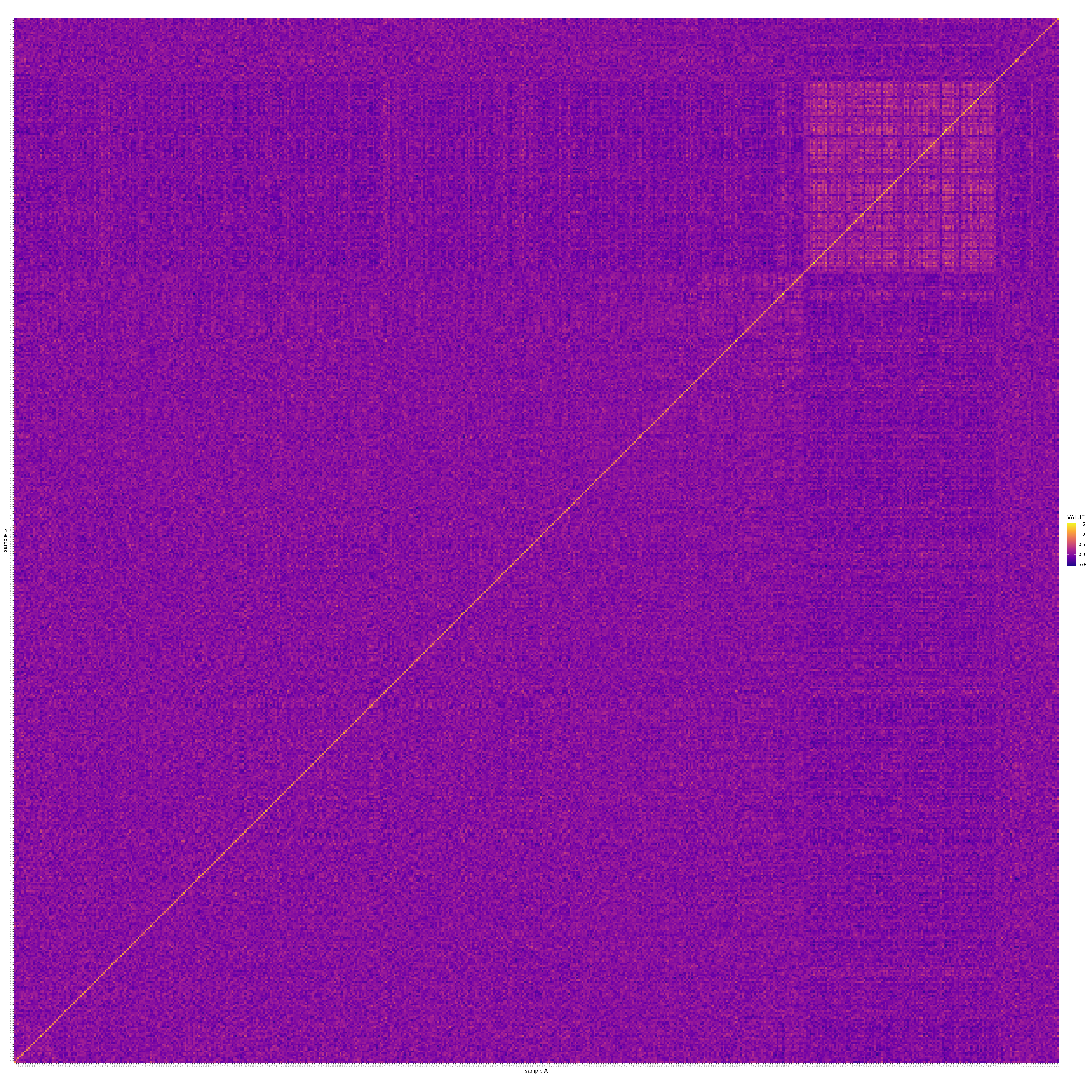
Finally, we used the called recombination blocks as pseudo-SNPs in an F₂-cross GWAS. To detect associations between the pseudo-SNPs and the two phenotypes of interest, we used a linear mixed model (LMM) as implemented in GCTA (Yang et al. 2011). For the genetic relationship matrix (GRM), we additionally used the leave-one-chromosome-out implementation of GCTA’s LMM, with excludes the chromosome on which the candidate SNP is located when calculating the GRM. A GRM constructed from the entire genome is presented as a heatmap in Figure 6.1, with each sample represented on each axis, and lighter colours representing a higher degree of relatedness between a pair of samples. The square in the top right-hand corner is created by samples ~550-648, which, based on Figure 5.4 above, clearly have distinct genotypes to the rest of the samples due to their having been bred from different F₁ parents.

Code

# Load libraries

library(tidyverse)
library(genio)

# Set variables

IN_PREF = "/hps/nobackup/birney/users/ian/somites/beds/F2/hdrr/None/5000/0.8"
LOW_COV = c(26, 89, 166, 178, 189, 227, 239, 470, 472, 473, 490, 501, 502, 503, 504, 505, 506, 507, 508, 509, 510, 511) %>% 
  as.character()

# Read in files

## Read bed
fam = genio::read_fam(IN_PREF)
bim = genio::read_bim(IN_PREF)
df_genos = genio::read_bed(IN_PREF,
                           names_loci = bim$id,
                           names_ind = fam$id) %>% 
  as.data.frame()


# Get indexes of all non-low coverage samples
ind_keep = which(!as.character(fam$id) %in% LOW_COV)
# Filter out low-cov samples from `fam` and `df_genos`
df_genos = df_genos[, ind_keep]
fam = fam %>% 
  dplyr::filter(!id %in% LOW_COV)

# Convert genos to matrix

x = df_genos %>% 
  # transpose
  t(.) %>% 
  # convert back to data frame
  as.data.frame(.)

# Compute GRM "manually"
# Following guidance here: https://zjuwhw.github.io/2021/08/20/GRM.html

n = dim(x)[1]
m = dim(x)[2]
# For each SNP, sum the ALT alleles and divide by 2n to get the ALT allele frequency
p_hat = apply(x, 2, sum)/(2*n)
# Standardise matrix by allele frequency
w = apply(rbind(x,p_hat), 2, function(x) (x-2*x[length(x)])/sqrt(2*x[length(x)]*(1-x[length(x)])))[1:n,]

# Cacluate the GRM
A = w %*% t(w) / m

#########################
# Plot GRM
#########################

# Order
ord = hclust(dist(A, method = "euclidean"), method = "ward.D")$order
#labs = rownames(A)[ord]
## Get labs with cross
#labs_x = tibble(SAMPLE = labs) %>% 
#  dplyr::left_join(f2 %>% 
#                     dplyr::select(SAMPLE, PAT_MAT),
#                   by = "SAMPLE") %>% 
#  # combine
#  dplyr::mutate(S_X = paste(SAMPLE, PAT_MAT, sep = "_"))

# Order matrix
A_ord = A[ord, ord]

# Convert to DF
df_fig = A_ord %>% 
  as.data.frame() %>% 
  tibble::rownames_to_column(var = "SAMPLE_1") %>% 
  tidyr::pivot_longer(-c(SAMPLE_1), names_to = "SAMPLE_2", values_to = "VALUE")

fig = df_fig %>% 
  ggplot() +
  geom_tile(aes(x = SAMPLE_1, y = SAMPLE_2, fill = VALUE)) +
  scale_fill_viridis_c(option = "plasma") +
  theme(aspect.ratio = 1) +
  theme(axis.text.x = element_text(angle = 90),
        axis.text = element_text(size = 2)) +
  xlab("sample A") +
  ylab("sample B")

fig

Figure 6.1: GRM generated for 600 F₂ samples using Equations @ref(eq:grmstd) and @ref(eq:grm). Code adapted from rule make_grm_man in https://github.com/brettellebi/somites/blob/master/workflow/rules/08_relationship_metrics.smk.

As described above in Chapter 2, the microscope used to image the embryos (either AU or DB) differed in heat by 0.7-0.8°C, which likely caused differences in the measurements observed. In an attempt to avoid complications resulting from its inclusion, we inverse-normalised the period phenotype within each microscope group, transforming the phenotype to fit a normal distribution across both microscopes (displayed in Figure 2.5). We only show the results from this transformed phenotype in the following section.

To set the significance threshold, we permuted the phenotype across samples using 10 different random seeds, together with all covariates when included, and ran a separate linkage model for each permutation. We then set the lowest \(p\)-value from all 10 permutation as the significance threshold for the non-permuted model. We additionally applied a Bonferroni correction to our \(p\)-values by dividing \(\alpha\) (0.05) by the number of pseudo-SNPs in the model, and set this as a secondary threshold.

6.2 Period intercept

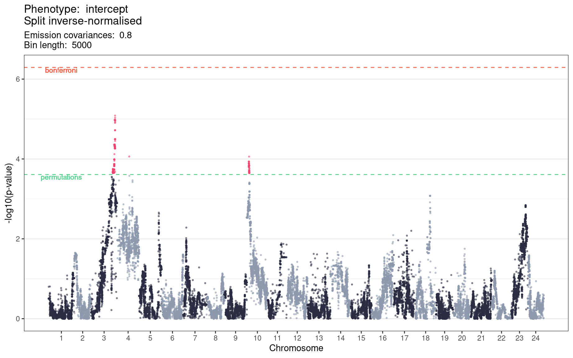
Figure 6.2 is a Manhattan plot of the genetic linkage results for the period intercept phenotype, inverse-normalised within microscopes as shown in Figure 2.5. The regions found to be significant based on the permutations’ minimum \(p\)-value are set out in Table 6.1.

Code

# Load libraries

library(tidyverse)

# Set variables

IN = "/hps/nobackup/birney/users/ian/somites/gcta/mlma_loco_invnorm/true/hdrr/None/5000/0.8/intercept.loco.mlma"
MIN_P = "/hps/nobackup/birney/users/ian/somites/gcta/mlma_loco_invnorm/min_p/hdrr/None/5000/0.8/intercept.csv"
BIN_LENGTH = 5000
COV = 0.8
PHENO = "intercept"

########################
# Plotting parameters
########################

gwas_pal = c("#2B2D42", "#F7B267", "#F25C54")
names(gwas_pal) = c("target", "even chr", "odd chr")

# Intercept
intercept_pal = c("#EF476F", "#8D99AE", "#2b2d42")
names(intercept_pal) = c("target", "even chr", "odd chr")

# PSM
unsegmented_psm_area_pal = c("#E59500", "#9C6FC3", "#401F3E")
names(unsegmented_psm_area_pal) = c("target", "even chr", "odd chr")

########################
# HdrR chromosome data
########################
# Get chromosome lengths
med_chr_lens = read.table(here::here("data",
                                     "Oryzias_latipes.ASM223467v1.dna.toplevel.fa_chr_counts.txt"),
                          col.names = c("chr", "end"))
# Add start
med_chr_lens$start = 1
# Reorder
med_chr_lens = med_chr_lens %>% 
  dplyr::select(chr, start, end) %>% 
  # remove MT
  dplyr::filter(chr != "MT") %>% 
  # convert to integer
  dplyr::mutate(chr = as.integer(chr)) %>% 
  # Add cumulative bases
  dplyr::mutate(CUMSUM = cumsum(end),
                TOT = CUMSUM - end) %>% 
  # Add midpoint for each chr
  dplyr::mutate(MID_TOT = TOT + (end / 2))

########################
# Read in files
########################

# Read in and process data

df = readr::read_tsv(IN) %>% 
  # Add POS
  dplyr::mutate(BIN_START = (bp * BIN_LENGTH) + 1,
                BIN_END = (bp + 1) * BIN_LENGTH) %>% 
  # join chromosome lengths
  dplyr::left_join(med_chr_lens, by = c("Chr" = "chr")) %>% 
  # add x-coord
  dplyr::mutate(X_COORD = BIN_START + TOT) %>% 
  # change column names
  dplyr::rename(CHROM = Chr)

# Get significance levels

## Permutations

PERM_SIG = readr::read_csv(MIN_P) %>% 
  dplyr::pull(MIN_P) %>% 
  min(.)

## Bonferroni

BONF_SIG = 0.05 / nrow(df)

# Set title

TITLE = paste("Phenotype: ",
              PHENO,
              "\nSplit inverse-normalised")

SUBTITLE = paste("Emission covariances: ",
                 COV,
                 "\nBin length: ",
                 BIN_LENGTH)

# Set palette

pal = eval(as.name(paste(PHENO, "_pal", sep = "")))

########################
# Manhattan plot function
########################

plot_man = function(df, title = NULL, subtitle = NULL, gwas_pal, size = 0.5, alpha = 0.5, med_chr_lens, perm_sig = NULL, bonf_sig = NULL){
  # Create palette
  pal = rep_len(gwas_pal, length.out = nrow(med_chr_lens))
  names(pal) = med_chr_lens$chr
  
  df = df %>% 
    # create `COLOUR` vector
    dplyr::mutate(COLOUR = dplyr::case_when(!is.null(perm_sig) & p < perm_sig ~ gwas_pal[1],
                                            gtools::even(CHROM) ~ gwas_pal[2],
                                            gtools::odd(CHROM) ~ gwas_pal[3])) %>% 
    dplyr::mutate(CHROM = factor(CHROM, levels = med_chr_lens$chr)) 
  
  out_plot = df %>% 
    ggplot(aes(x = X_COORD,
               y = -log10(p),
               label = BIN_START,
               label2 = BIN_END)) + 
    geom_point(colour = df$COLOUR,
               size = size,
               alpha = alpha) +
    #scale_color_manual(values = gwas_pal) +
    scale_x_continuous(breaks = med_chr_lens$MID_TOT, 
                       labels = med_chr_lens$chr) +
    theme_bw() +
    theme(panel.grid.major.x = element_blank(),
          panel.grid.minor.x = element_blank()
    ) +
    guides(colour = "none") +
    labs(title = title,
         subtitle = subtitle) +
    xlab("Chromosome") +
    ylab("-log10(p-value)") + 
    # permutations significance level
    geom_hline(yintercept = -log10(perm_sig), colour = "#60D394", linetype = "dashed") +
    geom_text(aes(MID_TOT[1], -log10(perm_sig), label = "permutations", vjust = 1), size = 3, colour = "#60D394") + 
    # bonferroni significance level
    geom_hline(yintercept = -log10(bonf_sig), colour = "#F06449", linetype = "dashed") +
    geom_text(aes(MID_TOT[1], -log10(bonf_sig), label = "bonferroni", vjust = 1), size = 3, colour = "#F06449")
  
  return(out_plot)
  
}

########################
# Plot and save
########################

# Plot
out_plot = plot_man(df,
                    title = TITLE,
                    subtitle = SUBTITLE,
                    gwas_pal = pal,
                    med_chr_lens = med_chr_lens,
                    perm_sig = PERM_SIG,
                    bonf_sig = BONF_SIG)

out_plot

Figure 6.2: Manhattan plot of the genetic linkage results for the period intercept phenotype, inverse-normalised across microscopes. Pseudo-SNPs with \(p\)-values lower than the permutation significance threshold are highlighted in red. Code adapted from rule get_manhattan_gcta_invnorm in https://github.com/brettellebi/somites/blob/master/workflow/rules/06_2_GWAS_GCTA_split_invnorm.smk.

Table 6.1: Significant 5-kb bin ranges for period intercept below the minimum p-value from 10 permutations.

Chromosome	Bin start	Bin end	Length (kb)
3	31880001	35420000	3540
4	18090001	18095000	5
10	2995001	3690000	695

These regions contained a total of 46,872 SNPs imputed from the genotype of the F₀ parental strains. We ran Ensembl’s Variant Effect Predictor (McLaren et al. 2016) over these SNPs to identify those that would be most likely to have functional consequences. The full counts of SNPs falling into each category of ‘consequence’ are set out in Table 6.2. From this process we identified 38 genes that included a missense variant, 1 that included a missense variant and a start lost (ENSORLG00000014616), and 1 that included a missense variant and a stop lost (ENSORLG00000015149).

Table 6.2: Variant Effect Predictor results for SNPs in the bins.

Consequence	Count
intron variant	47211
intergenic variant	20045
upstream gene variant	7304
downstream gene variant	5229
3 prime UTR variant	1082
synonymous variant	694
missense variant	383
5 prime UTR variant	201
splice region variant,intron variant	126
missense variant,splice region variant	19
splice region variant,synonymous variant	17
stop gained	3
splice donor variant	1
start lost	1
stop lost	1
stop lost,splice region variant	1

We then combined these results with bulk RNA-seq that they had performed on F₀ Cab and Kaga individuals, to determine which of these genes are expressed in the tail during embryogenesis. This allowed us to reduce to the list to 29 genes, and a gene ontology analysis of this found that the list of genes was enriched for body axis, somitogenesis, and segmentation (see table below). Using this list of genes, we are now in the process of knocking out the Cab allele in the Cab her7venus background to functionally validate whether any of these genes plays a role in setting the tempo of the segmentation clock.

Code

readr::read_csv(here::here("results/final_gene_list.csv")) %>% 
  # remove the 'Source:...' in square brackets
  dplyr::mutate(description = stringr::str_remove_all(description, "\\[.*\\]")) %>% 
  # rename columns
  dplyr::rename(Chromosome = "chromosome_name",
                `Ensembl gene ID` = "ensembl_gene_id",
                Description  = description) %>% 
  DT::datatable()

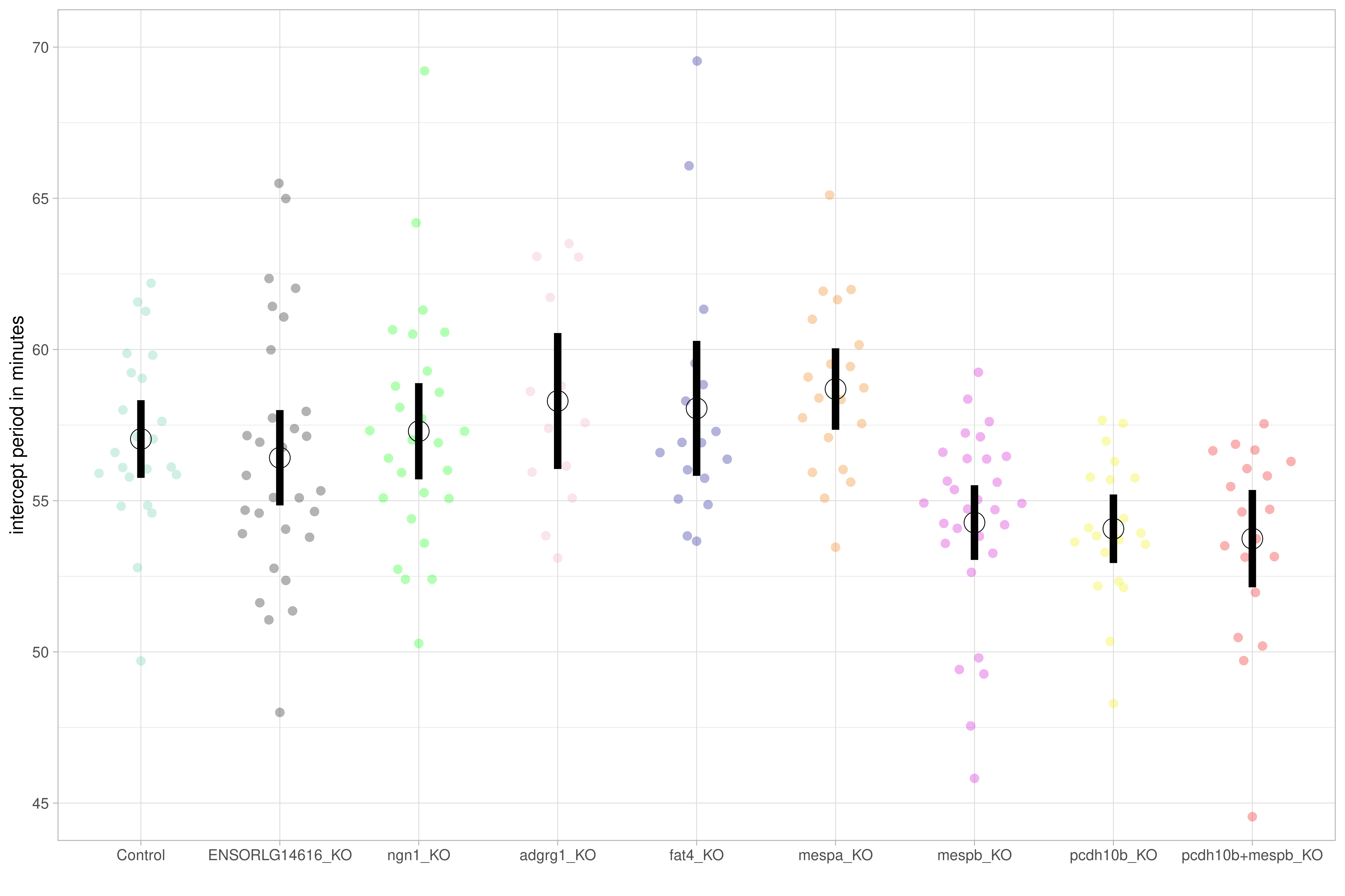
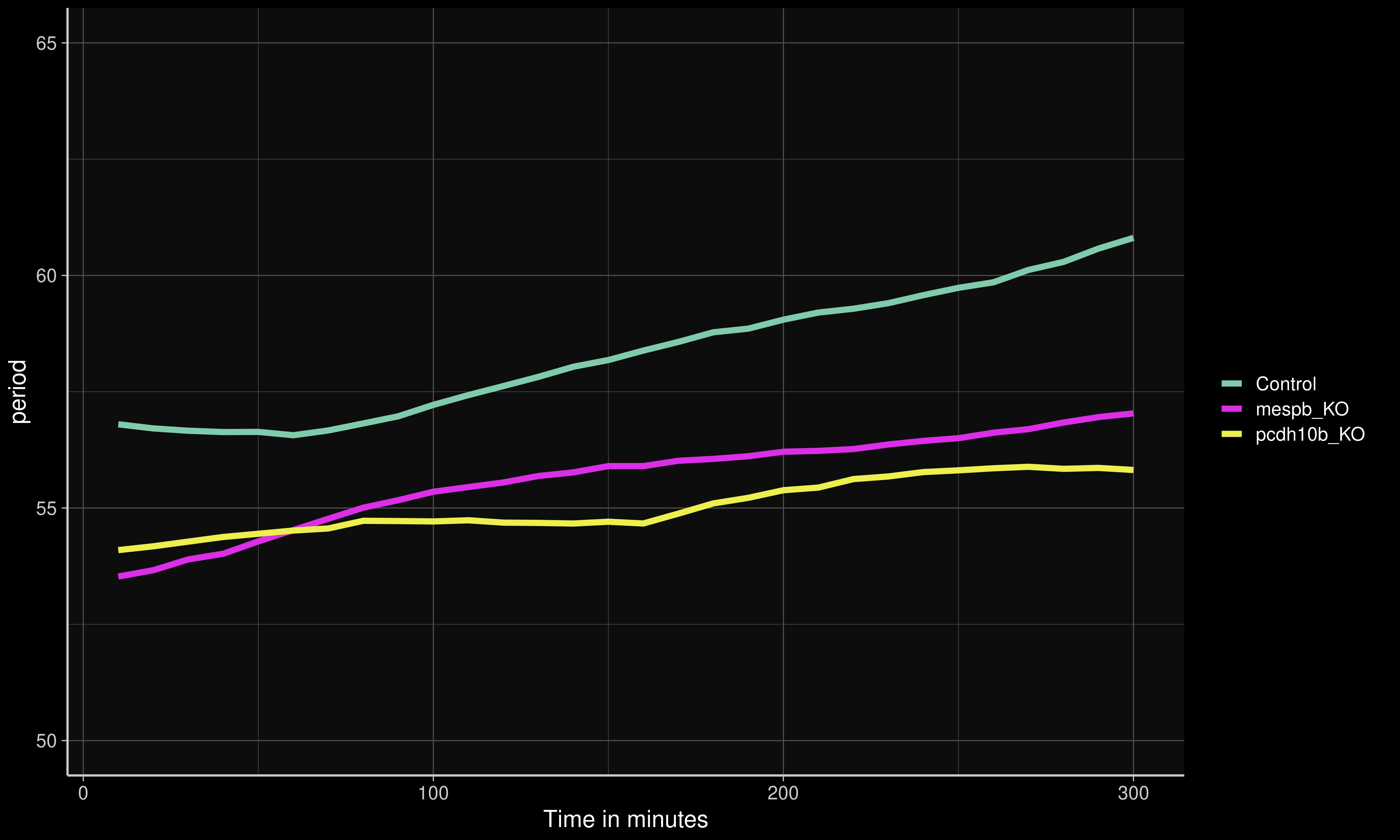
We have since begun the process of using the CRISPR-Cas9 system (Campenhout et al. 2019) to knock out some of these candidate genes to determine their effect on the period phenotype. The mespb (ENSORLG00000014656) and pcdh10b (ENSORLG00000020474) genes have both been found to be involved in segmental boundary formation and somite patterning (Hitachi et al. 2008; Rangarajan, Luo, and Sargent 2006), and are highly conserved in vertebrates (Gul et al. 2017; Satou, Imai, and Satoh 2004). Preliminary results have shown that knocking out either of these genes from the Cab strain significantly speeds up somite period development by 2-3 minutes (Figure 6.3 and Figure 6.4)), providing promising evidence that these genes are involved in the establishment of the segmentation clock.

book/plots/ali/20221123_email_attachments/Graph3.png

Figure 6.3: Period intercept for Cab embryos with CRISPR-Cas9 knock-outs (Campenhout et al. 2019) of mespb and pcdh10b compared to controls. Figure generated by Ali Seleit.

Figure 6.4: Mean period for Cab embryos with CRISPR-Cas9 knock-outs (Campenhout et al. 2019) of mespb and pcdh10b compared to controls. Figure generated by Ali Seleit.

6.3 PSM area

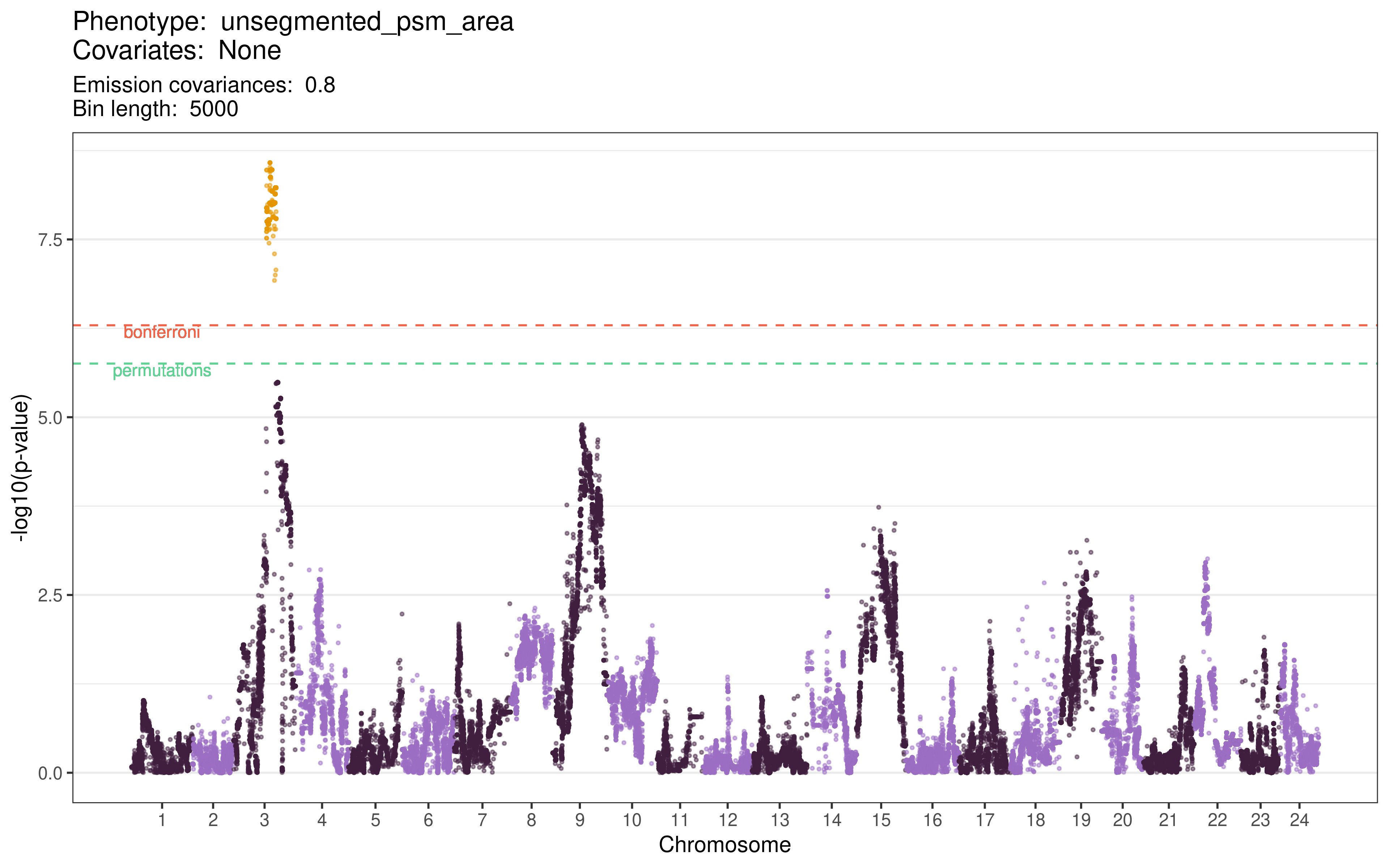
Figure 6.5 is a Manhattan plot of the genetic linkage results for the PSM area phenotype. The regions found to be significant based on the permutations’ minimum \(p\)-value are set out in the table below, although they exceed the Bonferroni correction threshold as well. I note that this ~6 Mb significant region on chromosome 3 does not overlap at all with the significant region discovered for the period intercept phenotype.

Figure 6.5: Manhattan plot of the genetic linkage results for the PSM area phenotype. Pseudo-SNPs with \(p\)-values lower than the permutation significance threshold are highlighted in yellow.

This region contained a total of 29,096 SNPs imputed from the genotype of the F₀ parental strains. I ran Ensembl’s Variant Effect Predictor (McLaren et al. 2016) over these SNPs to identify those that would be most likely to have functional consequences. The full counts of SNPs falling into each category of ‘consequence’ are set out in the table below.

From this process we identified 114 genes that included a missense variant, and 5 that included a both a missense variant and a splice region variant:

Code

readr::read_tsv(here::here("results/annotations_psm/hdrr/None/5000/0.8/unsegmented_psm_area/None/vep_out.txt"),
                comment = "##") %>% 
  dplyr::rename("Uploaded_variation" = "#Uploaded_variation") %>% 
  dplyr::filter(grepl("missense", Consequence)) %>% 
  dplyr::distinct(Gene, Consequence, .keep_all = T) %>% 
  DT::datatable(  )

We then combined these results with bulk RNA-seq that they had performed on F₀ Cab and Kaga individuals, to determine which of these genes are expressed in the unsegmented tail during embryogenesis. This allowed us to reduce to the list to 96 genes, although they were not apparently associated with a specific gene ontology as perhaps expected, given this is a single locus that is potentially driven by just one gene. As with the period intercept phenotype, we are now in the process of knocking out the Cab allele in the Cab her7venus background to assess if any of these genes play a role in determining the size of the PSM and to functionally validate the hits.

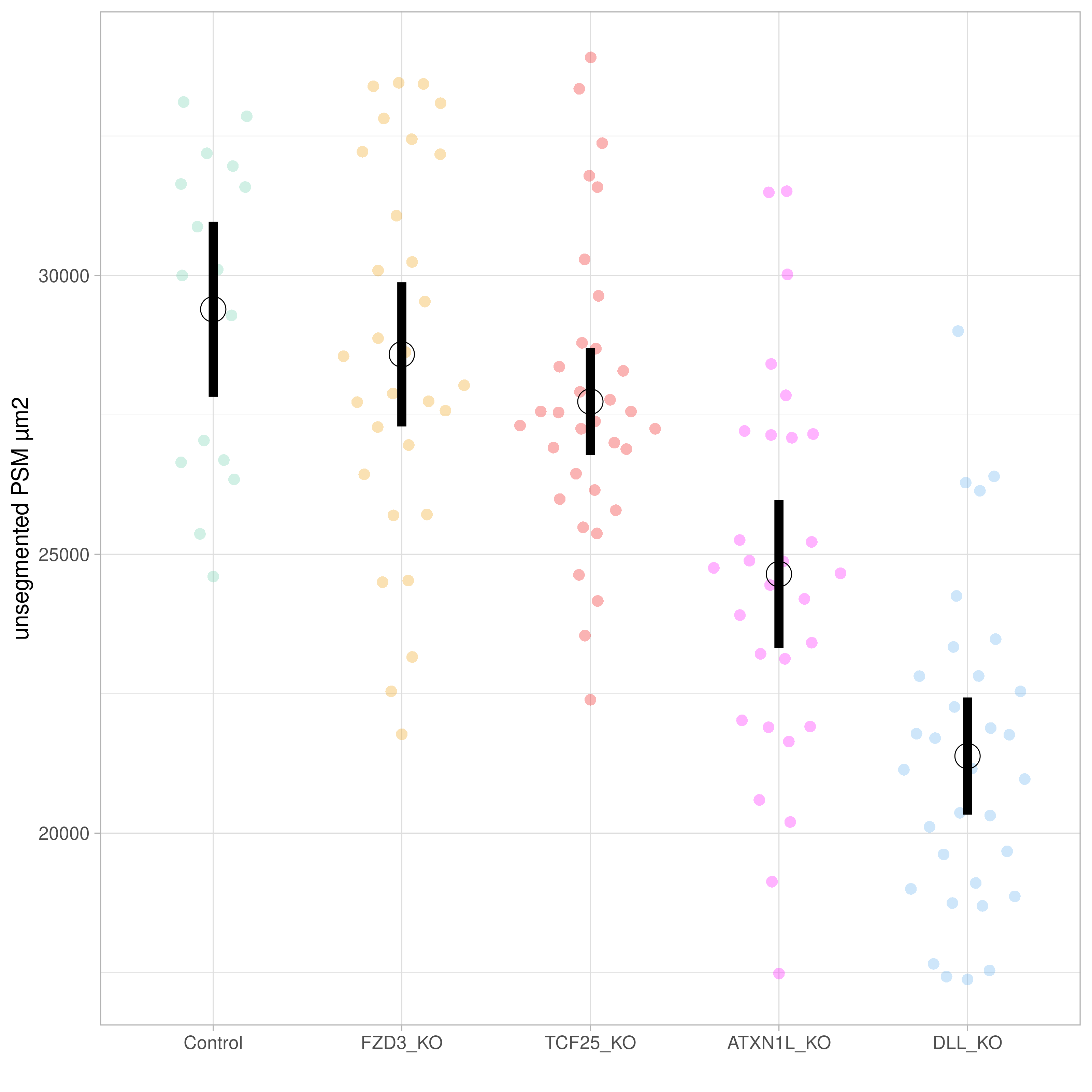
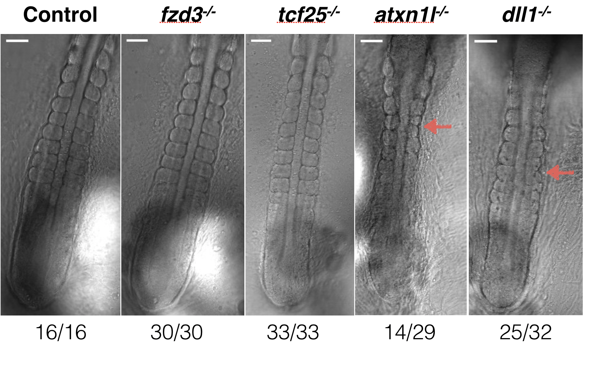
Two of these genes have shown a phenotype of reduced PSM area, segment boundary problems, and segment size (Figure 6.6 and Figure 6.7). The first, dll1, is a known player in somitogenesis. The second, atxn1l, has not been associated with somitogenesis before, but is a negative regulator of Notch signalling in mice and Drosophila (noting that Notch is a major player in segmentation in all vertebrates).

Figure 6.6: Unsegmented PSM area for Cab embryos with CRISPR-Cas9 knock-outs (Campenhout et al. 2019) of fzd3, tcf25, atxn1l and dll compared to controls. Figure generated by Ali Seleit.

Figure 6.7: Illustrative images of differences in somite segmentation for Cab embryos with CRISPR-Cas9 knock-outs (Campenhout et al. 2019) of fzd3, tcf25, atxn1l and dll1 compared to controls. The atxn1l and dll1 knock-outs show reduced PSM area, segment boundary problems, and segment size. Figure generated by Ali Seleit.

Campenhout, Claude Van, Pauline Cabochette, Anne-Clémence Veillard, Miklos Laczik, Agnieszka Zelisko-Schmidt, Céline Sabatel, Maxime Dhainaut, Benoit Vanhollebeke, Cyril Gueydan, and Véronique Kruys. 2019. “Guidelines for Optimized Gene Knockout Using CRISPR/Cas9.” BioTechniques 66 (6): 295–302. https://doi.org/10.2144/btn-2018-0187.

Gul, Ismail Sahin, Paco Hulpiau, Yvan Saeys, and Frans van Roy. 2017. “Evolution and Diversity of Cadherins and Catenins.” Experimental Cell Research, Cell Sensing and Signaling via Cell-Cell Adhesion, 358 (1): 3–9. https://doi.org/10.1016/j.yexcr.2017.03.001.

Hitachi, Keisuke, Hiroki Danno, Akiko Kondow, Kiyoshi Ohnuma, Hideho Uchiyama, Shoichi Ishiura, Akira Kurisaki, and Makoto Asashima. 2008. “Physical Interaction Between Tbx6 and Mespb Is Indispensable for the Activation of Bowline Expression During Xenopus Somitogenesis.” Biochemical and Biophysical Research Communications 372 (4): 607–12. https://doi.org/10.1016/j.bbrc.2008.05.083.

McLaren, William, Laurent Gil, Sarah E. Hunt, Harpreet Singh Riat, Graham R. S. Ritchie, Anja Thormann, Paul Flicek, and Fiona Cunningham. 2016. “The Ensembl Variant Effect Predictor.” Genome Biology 17 (1): 122. https://doi.org/10.1186/s13059-016-0974-4.

Rangarajan, Janaki, Ting Luo, and Thomas D. Sargent. 2006. “PCNS: A Novel Protocadherin Required for Cranial Neural Crest Migration and Somite Morphogenesis in Xenopus.” Developmental Biology 295 (1): 206–18. https://doi.org/10.1016/j.ydbio.2006.03.025.

Satou, Yutaka, Kaoru S. Imai, and Nori Satoh. 2004. “The Ascidian Mesp Gene Specifies Heart Precursor Cells.” Development 131 (11): 2533–41. https://doi.org/10.1242/dev.01145.

Yang, Jian, S. Hong Lee, Michael E. Goddard, and Peter M. Visscher. 2011. “GCTA: A Tool for Genome-wide Complex Trait Analysis.” The American Journal of Human Genetics 88 (1): 76–82. https://doi.org/10.1016/j.ajhg.2010.11.011.