3  F0 homozygosity

3.1 F0 coverage

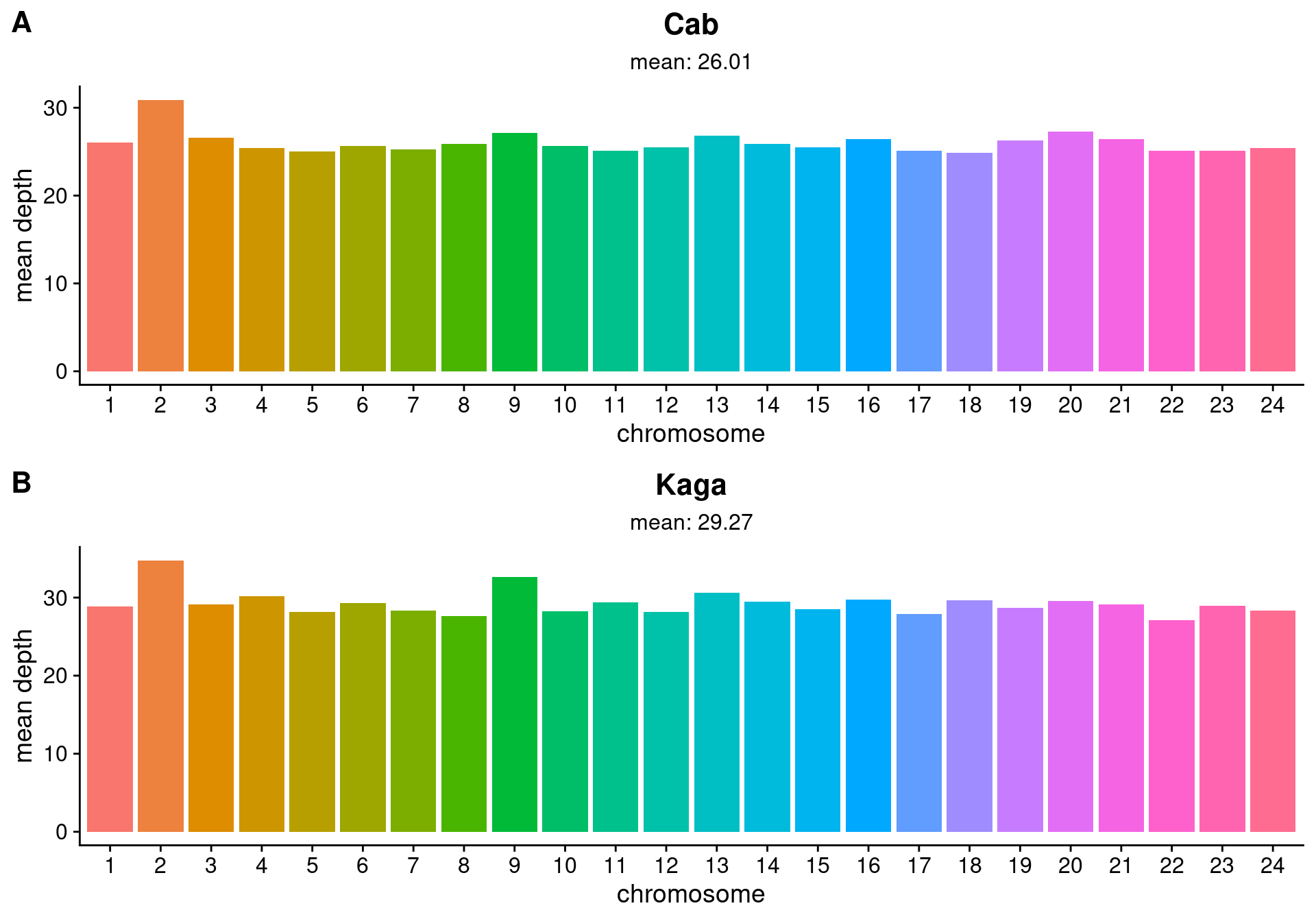
Ali Seleit extracted DNA from the F0, F1, and F2, and sequenced the F0 and F1 samples with the Illumina platform at high coverage (~26x for Cab and ~29x for Kaga), as measured by SAMtools (Danecek et al. 2021). Figure 3.1 sets out the mean sequencing depth within each chromosome and across the whole genome for the Cab and Kaga F0 samples. We then sequenced the F2 samples at low coverage (~1x), which would be sufficient to map their genotypes back to the genotypes of their parental strains (see Chapter 5 for further details).

Code
# Set variables

IN = list.files("/hps/nobackup/birney/users/ian/somites/coverage/hdrr/bwamem2",
                     full.names = T) %>% 
  as.list()
OUT_PNG = "/hps/software/users/birney/ian/repos/somites/book/plots/coverage/F0_coverage.png"
OUT_PDF = "/hps/software/users/birney/ian/repos/somites/book/plots/coverage/F0_coverage.pdf"

# Read in files

names(IN) = IN %>% 
  unlist() %>% 
  basename() %>% 
  stringr::str_remove(".txt")

dat_list = purrr::map(IN, function(FILE){
  readr::read_tsv(FILE) %>% 
    dplyr::rename(chrom = '#rname') %>% 
    dplyr::filter(chrom != "MT") %>% 
    dplyr::mutate(chrom = factor(chrom, levels = 1:24))
})

# Plot

fig_cab = dat_list[["Cab"]] %>% 
  ggplot() + 
  geom_col(aes(chrom, meandepth, fill = chrom)) + 
  cowplot::theme_cowplot() +
  #facet_wrap(~SAMPLE, nrow = 2) + 
  scale_x_discrete(breaks = 1:24) +
  guides(fill = "none") +
  xlab("chromosome") +
  ylab("mean depth") +
  ggtitle("Cab",
          subtitle = paste("mean: ", 
                           round(mean(dat_list[["Cab"]]$meandepth),
                                 digits = 2),
                           sep = "")
          ) + 
  theme(plot.title = element_text(hjust = 0.5),
        plot.subtitle = element_text(hjust = 0.5))

fig_kaga = dat_list[["Kaga"]] %>% 
  ggplot() + 
  geom_col(aes(chrom, meandepth, fill = chrom)) + 
  cowplot::theme_cowplot() +
  #facet_wrap(~SAMPLE, nrow = 2) + 
  scale_x_discrete(breaks = 1:24) +
  guides(fill = "none") +
  xlab("chromosome") +
  ylab("mean depth") +
  ggtitle("Kaga",
          subtitle = paste("mean: ", 
                           round(mean(dat_list[["Kaga"]]$meandepth),
                                 digits = 2),
                           sep = "")
  ) + 
  theme(plot.title = element_text(hjust = 0.5),
        plot.subtitle = element_text(hjust = 0.5))


# Put together

out = cowplot::plot_grid(fig_cab,
                         fig_kaga,
                         align = "hv",
                         axis = "tblr",nrow = 2,labels = c("A", "B"),label_size = 16)

out

Figure 3.1: Mean sequencing depth per chromosome for Cab and Kaga F0 strains, with genome-wide mean depth across all chromosomes shown under the subtitles. Code adapted from rule coverage_plot_F0 in https://github.com/brettellebi/somites/blob/master/workflow/rules/08_extra.smk.

3.2 F0 homozygosity

Before proceeding to map the F2 sequences to the genotypes of the F0 generation, we first investigated the levels of homozygosity in the F0 Cab and Kaga strains, as this would affect our ability to accurately call the F2 generation. That is to say, for regions where either F0 parent is consistently heterozygous, it would be difficult to determine the parent from which a particular F2 individual derived its chromosomes at that locus. We therefore aligned the high-coverage sequencing data for the F0 Cab and Kaga strains to the medaka HdrR reference (Ensembl release 104, build ASM223467v1) using BWA-MEM2 (Vasimuddin et al. 2019), sorted the aligned .sam files, marked duplicate reads, and merged the paired reads with picard (“Picard Toolkit” 2019), and indexed the .bam files with SAMtools (Li et al. 2009). The Snakemake modules used to map and align these samples are set out here and here.

To call variants, we followed the GATK best practices (to the extent they were applicable) (McKenna et al. 2010; DePristo et al. 2011; Van der Auwera and O’Connor 2020) with GATK’s HaplotypeCaller and GenotypeGVCFs tools (Poplin et al. 2018), then merged all calls into a single .vcf file with picard (“Picard Toolkit” 2019). Finally, we extracted the biallelic calls for Cab and Kaga with bcftools (Danecek et al. 2021), counted the number of SNPs within non-overlapping, 5-kb bins, and calculated the proportion of SNPs within each bin that were homozygous.

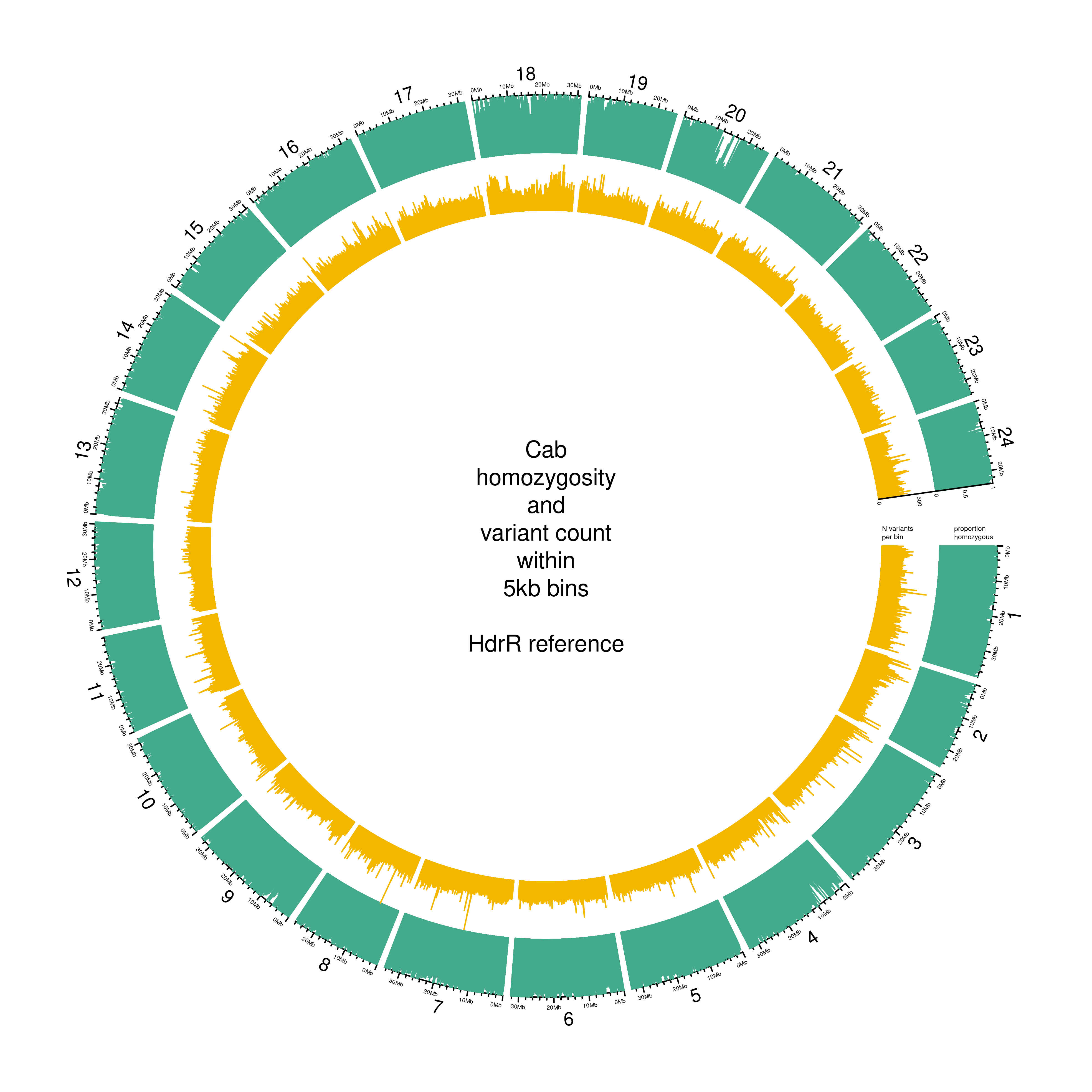
Figure 3.2 is a circos plot generated with circlize (Gu et al. 2014) for the Cab F0 strain used in this experiment, featuring the proportion of homozygous SNPs per 5-kb bin (green), and the total number of SNPs in each bin (yellow). As expected for a strain that has been inbred for over 10 generations, the mean homozygosity for this strain is high, with a mean proportion of homozygosity across all bins of 83%.

Code
# Load libraries

library(tidyverse)
library(circlize)

# Set variables

IN_FILE = "/hps/nobackup/birney/users/ian/somites/genos/F0_and_F1/hdrr/counts/Cab/5000.csv"
CHROM_LENGTHS = here::here("config/hdrr_chrom_lengths.csv")
REF = "hdrr"
SAMPLE = "Cab"
BIN_LENGTH = 5000
PAL = "#43AA8B"
OUT_PNG = here::here("book/plots/circos/trio_homo/hdrr/5000/Cab.png")


# Get lighter/darker functions

source("https://gist.githubusercontent.com/brettellebi/c5015ee666cdf8d9f7e25fa3c8063c99/raw/91e601f82da6c614b4983d8afc4ef399fa58ed4b/karyoploteR_lighter_darker.R")


# Read in data

genos = readr::read_csv(IN_FILE)

chroms = readr::read_csv(CHROM_LENGTHS,
                         col_names = c("CHROM", "LENGTH")) %>% 
  # remove MT
  dplyr::filter(CHROM != "MT") %>% 
  dplyr::mutate(CHROM = CHROM %>% 
                  stringr::str_replace(pattern = "^", replacement = "chr"),
                START = 1) %>% 
  dplyr::select(CHROM, START, END = LENGTH)

# Process variables

if (SAMPLE == "F1"){
  TARGET_CHROM = "PROP_HET"
} else {
  TARGET_CHROM = "PROP_HOM"
}

if (REF == "hdrr"){
  REF = "HdrR"
} else if (REF == "hni"){
  REF = "HNI"
}

# Process `genos`

homozyg = genos %>% 
  dplyr::mutate(CHROM = CHROM %>% 
                  stringr::str_replace(pattern = "^", replacement = "chr"),
                BIN_START = (BIN -1) * BIN_LENGTH + 1,
                BIN_END = BIN * BIN_LENGTH) %>% 
  dplyr::select(CHROM, BIN_START, BIN_END, dplyr::all_of(TARGET_CHROM))

n_vars = genos %>% 
  dplyr::mutate(CHROM = CHROM %>% 
                  stringr::str_replace(pattern = "^", replacement = "chr"),
                BIN_START = (BIN -1) * BIN_LENGTH + 1,
                BIN_END = BIN * BIN_LENGTH) %>% 
  dplyr::select(CHROM, BIN_START, BIN_END, TOT_HITS) 

########################
# PNG
########################

# Set output

png(OUT_PNG,
    width = 20,
    height = 20,
    units = "cm",
    res = 500)

# Create Circos plots

circos.par(cell.padding = c(0, 0, 0, 0),
           track.margin = c(0, 0),
           gap.degree = c(rep(1, nrow(chroms) - 1), 8))

# Initialize plot

circos.initializeWithIdeogram(chroms,
                              plotType = c("axis", "labels"),
                              major.by = 1e7,
                              axis.labels.cex = 0.25*par("cex"))

if (SAMPLE == "F1"){
  CENTER_LAB = paste(SAMPLE,
                     "\nheterozygosity\nand\nvariant count",
                     "\nwithin\n",
                     BIN_LENGTH / 1000,
                     "kb bins",
                     "\n\n",
                     REF,
                     " reference",
                     sep = "")
} else {
  CENTER_LAB = paste(SAMPLE,
                     "\nhomozygosity\nand\nvariant count",
                     "\nwithin\n",
                     BIN_LENGTH / 1000,
                     "kb bins",
                     "\n\n",
                     REF,
                     " reference",
                     sep = "")
}
# Add label to center
text(0, 0, CENTER_LAB)

# Add proportion of homozygosity

circos.genomicTrack(homozyg,
                    panel.fun = function(region, value, ...) {
                      circos.genomicLines(region,
                                          value,
                                          type = "h",
                                          col = PAL,
                                          cex = 0.05)
                    },
                    track.height = 0.12,
                    bg.border = NA,
                    ylim = c(0, 1))
# y-axis label
circos.yaxis(side = "right",
             at = c(0, 0.5, 1),
             labels.cex = 0.25*par("cex"),
             tick.length = 2
)
# y-axis title

if (SAMPLE == "F1"){
  AXIS_LAB = "proportion\nheterozygous"
} else {
  AXIS_LAB = "proportion\nhomozygous"
}

circos.text(0, 0.25,
            labels = AXIS_LAB,
            sector.index = "chr1",
            facing = "clockwise",
            adj = c(0, -0.5),
            cex = 0.3*par("cex"))

# Add number of hits

## get max number of variants

MAX_VARS = max(n_vars$TOT_HITS, na.rm = T)

circos.genomicTrack(n_vars,
                    panel.fun = function(region, value, ...) {
                      circos.genomicLines(region,
                                          value,
                                          type = "h",
                                          col = "#F3B700",
                                          cex = 0.05)
                    },
                    track.height = 0.12,
                    bg.border = NA,
                    ylim = c(0, MAX_VARS))
# y-axis label
circos.yaxis(side = "right",
             at = c(0, 500),
             labels.cex = 0.25*par("cex"),
             tick.length = 2
)

circos.text(0, 0,
            labels = "N variants\nper bin",
            sector.index = "chr1",
            facing = "clockwise",
            adj = c(0, -0.5),
            cex = 0.3*par("cex"))

dev.off()

Figure 3.2: Proportion of homozygous SNPs within 5 kb bins in the Cab F0 generation genome (green), and number of SNPs in each bin (yellow). Code set out in rule circos_homozygosity in https://github.com/brettellebi/somites/blob/master/workflow/rules/04_trio_homozygosity.smk.

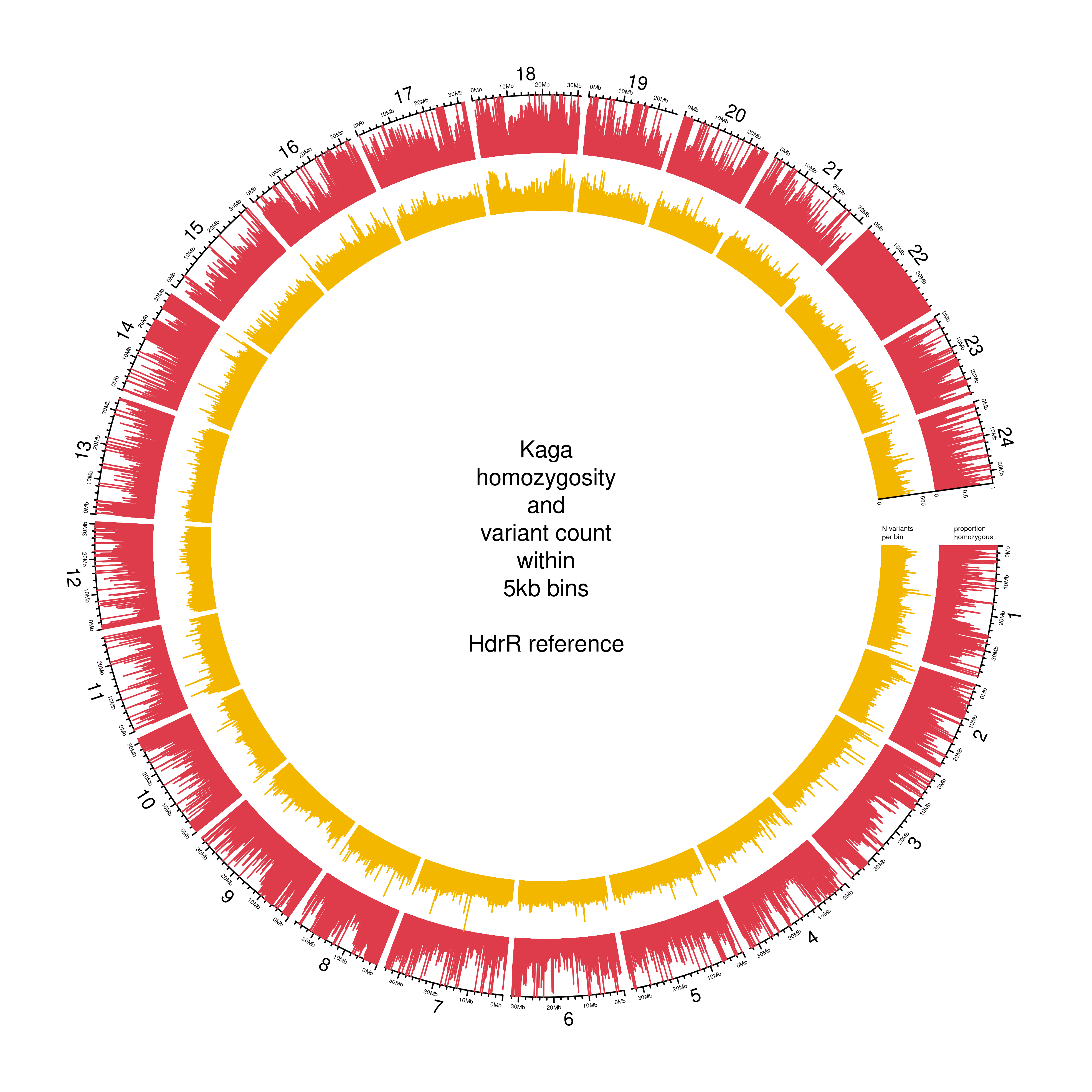
However, the levels of homozygosity in the Kaga strain used in this experiment was far lower, with a mean homozygosity across all bins of only 31% (Figure 3.3). This was a surprise, as it is an established strain that has been extant for decades, and we therefore expected the level of homozygosity to be commensurate with that observed in the Cab strain. An obvious exception is chr22, for which Kaga appears to be homozygous across its entire length.

Code
# Load libraries

library(tidyverse)
library(circlize)

# Set variables

IN_FILE = "/hps/nobackup/birney/users/ian/somites/genos/F0_and_F1/hdrr/counts/Kaga/5000.csv"
CHROM_LENGTHS = here::here("config/hdrr_chrom_lengths.csv")
REF = "hdrr"
SAMPLE = "Kaga"
BIN_LENGTH = 5000
PAL = "#DE3C4B"
OUT_PNG = here::here("book/plots/circos/trio_homo/hdrr/5000/Kaga.png")


# Get lighter/darker functions

source("https://gist.githubusercontent.com/brettellebi/c5015ee666cdf8d9f7e25fa3c8063c99/raw/91e601f82da6c614b4983d8afc4ef399fa58ed4b/karyoploteR_lighter_darker.R")


# Read in data

genos = readr::read_csv(IN_FILE)

chroms = readr::read_csv(CHROM_LENGTHS,
                         col_names = c("CHROM", "LENGTH")) %>% 
  # remove MT
  dplyr::filter(CHROM != "MT") %>% 
  dplyr::mutate(CHROM = CHROM %>% 
                  stringr::str_replace(pattern = "^", replacement = "chr"),
                START = 1) %>% 
  dplyr::select(CHROM, START, END = LENGTH)

# Process variables

if (SAMPLE == "F1"){
  TARGET_CHROM = "PROP_HET"
} else {
  TARGET_CHROM = "PROP_HOM"
}

if (REF == "hdrr"){
  REF = "HdrR"
} else if (REF == "hni"){
  REF = "HNI"
}

# Process `genos`

homozyg = genos %>% 
  dplyr::mutate(CHROM = CHROM %>% 
                  stringr::str_replace(pattern = "^", replacement = "chr"),
                BIN_START = (BIN -1) * BIN_LENGTH + 1,
                BIN_END = BIN * BIN_LENGTH) %>% 
  dplyr::select(CHROM, BIN_START, BIN_END, dplyr::all_of(TARGET_CHROM))

n_vars = genos %>% 
  dplyr::mutate(CHROM = CHROM %>% 
                  stringr::str_replace(pattern = "^", replacement = "chr"),
                BIN_START = (BIN -1) * BIN_LENGTH + 1,
                BIN_END = BIN * BIN_LENGTH) %>% 
  dplyr::select(CHROM, BIN_START, BIN_END, TOT_HITS) 

########################
# PNG
########################

# Set output

png(OUT_PNG,
    width = 20,
    height = 20,
    units = "cm",
    res = 500)

# Create Circos plots

circos.par(cell.padding = c(0, 0, 0, 0),
           track.margin = c(0, 0),
           gap.degree = c(rep(1, nrow(chroms) - 1), 8))

# Initialize plot

circos.initializeWithIdeogram(chroms,
                              plotType = c("axis", "labels"),
                              major.by = 1e7,
                              axis.labels.cex = 0.25*par("cex"))

if (SAMPLE == "F1"){
  CENTER_LAB = paste(SAMPLE,
                     "\nheterozygosity\nand\nvariant count",
                     "\nwithin\n",
                     BIN_LENGTH / 1000,
                     "kb bins",
                     "\n\n",
                     REF,
                     " reference",
                     sep = "")
} else {
  CENTER_LAB = paste(SAMPLE,
                     "\nhomozygosity\nand\nvariant count",
                     "\nwithin\n",
                     BIN_LENGTH / 1000,
                     "kb bins",
                     "\n\n",
                     REF,
                     " reference",
                     sep = "")
}
# Add label to center
text(0, 0, CENTER_LAB)

# Add proportion of homozygosity

circos.genomicTrack(homozyg,
                    panel.fun = function(region, value, ...) {
                      circos.genomicLines(region,
                                          value,
                                          type = "h",
                                          col = PAL,
                                          cex = 0.05)
                    },
                    track.height = 0.12,
                    bg.border = NA,
                    ylim = c(0, 1))
# y-axis label
circos.yaxis(side = "right",
             at = c(0, 0.5, 1),
             labels.cex = 0.25*par("cex"),
             tick.length = 2
)
# y-axis title

if (SAMPLE == "F1"){
  AXIS_LAB = "proportion\nheterozygous"
} else {
  AXIS_LAB = "proportion\nhomozygous"
}

circos.text(0, 0.25,
            labels = AXIS_LAB,
            sector.index = "chr1",
            facing = "clockwise",
            adj = c(0, -0.5),
            cex = 0.3*par("cex"))

# Add number of hits

## get max number of variants

MAX_VARS = max(n_vars$TOT_HITS, na.rm = T)

circos.genomicTrack(n_vars,
                    panel.fun = function(region, value, ...) {
                      circos.genomicLines(region,
                                          value,
                                          type = "h",
                                          col = "#F3B700",
                                          cex = 0.05)
                    },
                    track.height = 0.12,
                    bg.border = NA,
                    ylim = c(0, MAX_VARS))
# y-axis label
circos.yaxis(side = "right",
             at = c(0, 500),
             labels.cex = 0.25*par("cex"),
             tick.length = 2
)

circos.text(0, 0,
            labels = "N variants\nper bin",
            sector.index = "chr1",
            facing = "clockwise",
            adj = c(0, -0.5),
            cex = 0.3*par("cex"))

dev.off()

Figure 3.3: Proportion of homozygous SNPs within 5 kb bins in the Kaga F0 generation genome (red), and number of SNPs in each bin (yellow). Code set out in rule circos_homozygosity in https://github.com/brettellebi/somites/blob/master/workflow/rules/04_trio_homozygosity.smk

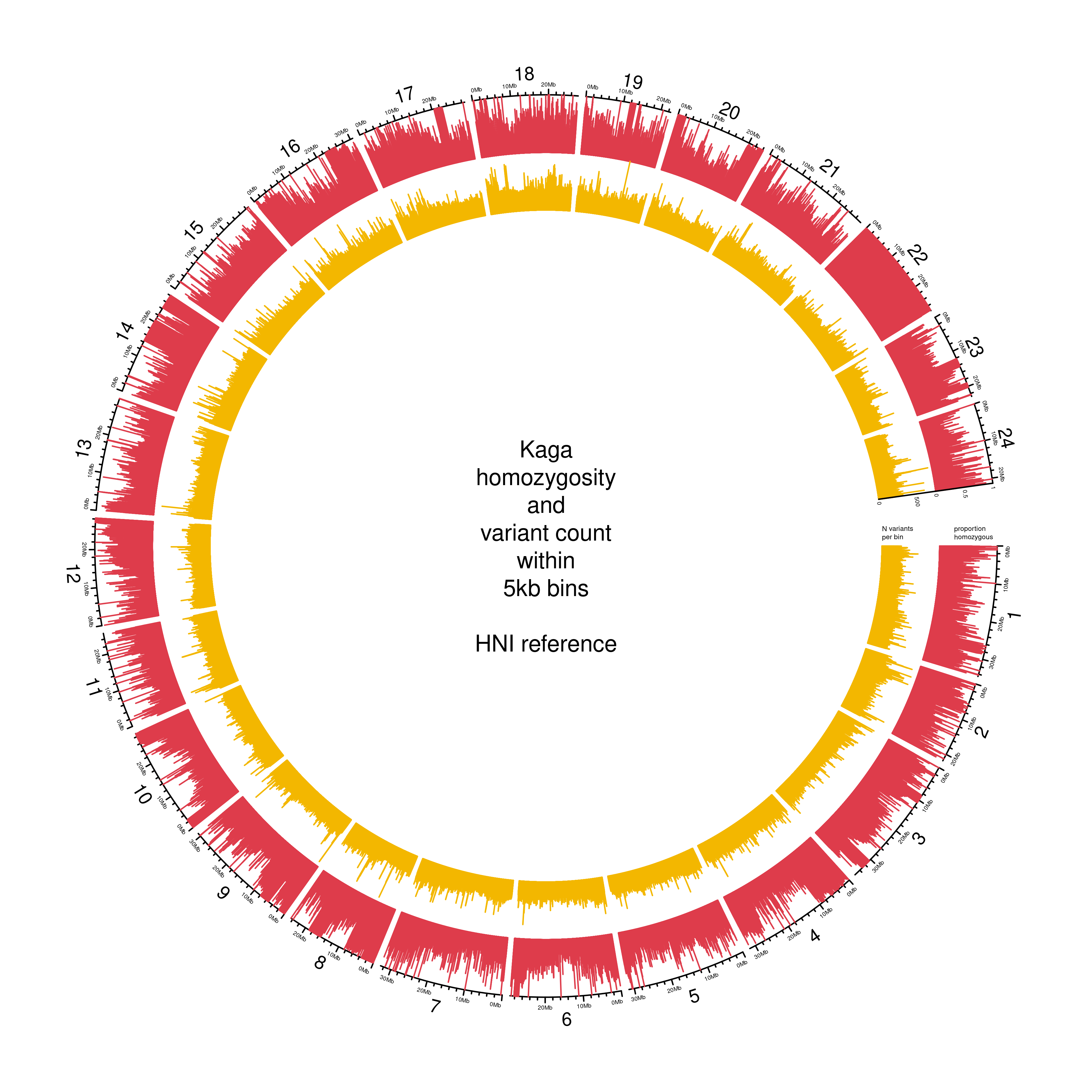
To determine whether the low levels of observed homozygosity in Kaga was affected by its alignments to the southern Japanese HdrR reference, we also aligned the F0 samples to the northern Japanese HNI reference (Figure 3.4). This did not make differences to the levels of observed homozygosity in either sample, which gave us confidence that the low homozygosity observed in Kaga was not driven by reference bias. The low homozygosity of this Kaga individual must have resulted from the strain having been contaminated at some stage by breeding with a different inbred strain prior to when they received the individuals.

Code
# Load libraries

library(tidyverse)
library(circlize)

# Set variables

IN_FILE = "/hps/nobackup/birney/users/ian/somites/genos/F0_and_F1/hni/counts/Kaga/5000.csv"
CHROM_LENGTHS = here::here("config/hdrr_chrom_lengths.csv")
REF = "hni"
SAMPLE = "Kaga"
BIN_LENGTH = 5000
PAL = "#DE3C4B"
OUT_PNG = here::here("book/plots/circos/trio_homo/hni/5000/Kaga.png")


# Get lighter/darker functions

source("https://gist.githubusercontent.com/brettellebi/c5015ee666cdf8d9f7e25fa3c8063c99/raw/91e601f82da6c614b4983d8afc4ef399fa58ed4b/karyoploteR_lighter_darker.R")


# Read in data

genos = readr::read_csv(IN_FILE)

chroms = readr::read_csv(CHROM_LENGTHS,
                         col_names = c("CHROM", "LENGTH")) %>% 
  # remove MT
  dplyr::filter(CHROM != "MT") %>% 
  dplyr::mutate(CHROM = CHROM %>% 
                  stringr::str_replace(pattern = "^", replacement = "chr"),
                START = 1) %>% 
  dplyr::select(CHROM, START, END = LENGTH)

# Process variables

if (SAMPLE == "F1"){
  TARGET_CHROM = "PROP_HET"
} else {
  TARGET_CHROM = "PROP_HOM"
}

if (REF == "hdrr"){
  REF = "HdrR"
} else if (REF == "hni"){
  REF = "HNI"
}

# Process `genos`

homozyg = genos %>% 
  dplyr::mutate(CHROM = CHROM %>% 
                  stringr::str_replace(pattern = "^", replacement = "chr"),
                BIN_START = (BIN -1) * BIN_LENGTH + 1,
                BIN_END = BIN * BIN_LENGTH) %>% 
  dplyr::select(CHROM, BIN_START, BIN_END, dplyr::all_of(TARGET_CHROM))

n_vars = genos %>% 
  dplyr::mutate(CHROM = CHROM %>% 
                  stringr::str_replace(pattern = "^", replacement = "chr"),
                BIN_START = (BIN -1) * BIN_LENGTH + 1,
                BIN_END = BIN * BIN_LENGTH) %>% 
  dplyr::select(CHROM, BIN_START, BIN_END, TOT_HITS) 

########################
# PNG
########################

# Set output

png(OUT_PNG,
    width = 20,
    height = 20,
    units = "cm",
    res = 500)

# Create Circos plots

circos.par(cell.padding = c(0, 0, 0, 0),
           track.margin = c(0, 0),
           gap.degree = c(rep(1, nrow(chroms) - 1), 8))

# Initialize plot

circos.initializeWithIdeogram(chroms,
                              plotType = c("axis", "labels"),
                              major.by = 1e7,
                              axis.labels.cex = 0.25*par("cex"))

if (SAMPLE == "F1"){
  CENTER_LAB = paste(SAMPLE,
                     "\nheterozygosity\nand\nvariant count",
                     "\nwithin\n",
                     BIN_LENGTH / 1000,
                     "kb bins",
                     "\n\n",
                     REF,
                     " reference",
                     sep = "")
} else {
  CENTER_LAB = paste(SAMPLE,
                     "\nhomozygosity\nand\nvariant count",
                     "\nwithin\n",
                     BIN_LENGTH / 1000,
                     "kb bins",
                     "\n\n",
                     REF,
                     " reference",
                     sep = "")
}
# Add label to center
text(0, 0, CENTER_LAB)

# Add proportion of homozygosity

circos.genomicTrack(homozyg,
                    panel.fun = function(region, value, ...) {
                      circos.genomicLines(region,
                                          value,
                                          type = "h",
                                          col = PAL,
                                          cex = 0.05)
                    },
                    track.height = 0.12,
                    bg.border = NA,
                    ylim = c(0, 1))
# y-axis label
circos.yaxis(side = "right",
             at = c(0, 0.5, 1),
             labels.cex = 0.25*par("cex"),
             tick.length = 2
)
# y-axis title

if (SAMPLE == "F1"){
  AXIS_LAB = "proportion\nheterozygous"
} else {
  AXIS_LAB = "proportion\nhomozygous"
}

circos.text(0, 0.25,
            labels = AXIS_LAB,
            sector.index = "chr1",
            facing = "clockwise",
            adj = c(0, -0.5),
            cex = 0.3*par("cex"))

# Add number of hits

## get max number of variants

MAX_VARS = max(n_vars$TOT_HITS, na.rm = T)

circos.genomicTrack(n_vars,
                    panel.fun = function(region, value, ...) {
                      circos.genomicLines(region,
                                          value,
                                          type = "h",
                                          col = "#F3B700",
                                          cex = 0.05)
                    },
                    track.height = 0.12,
                    bg.border = NA,
                    ylim = c(0, MAX_VARS))
# y-axis label
circos.yaxis(side = "right",
             at = c(0, 500),
             labels.cex = 0.25*par("cex"),
             tick.length = 2
)

circos.text(0, 0,
            labels = "N variants\nper bin",
            sector.index = "chr1",
            facing = "clockwise",
            adj = c(0, -0.5),
            cex = 0.3*par("cex"))

dev.off()

Figure 3.4: Proportion of homozygous SNPs within 5 kb bins in the Kaga F0 generation genome when aligned to the HNI reference (red), and number of SNPs in each bin (yellow). Code adapted from rule circos_homozygosity in https://github.com/brettellebi/somites/blob/master/workflow/rules/04_trio_homozygosity.smk.