4  F₁ heterozygosity

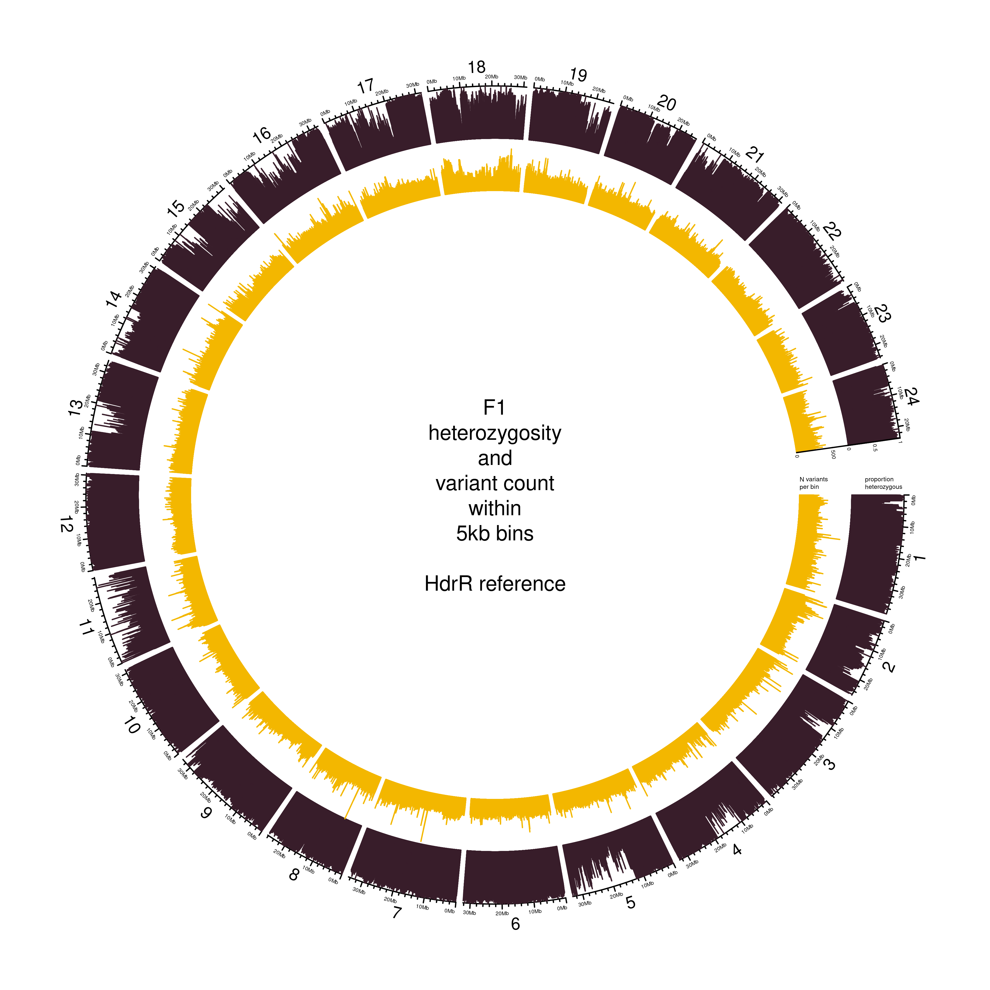
We next examined the level of heterozygosity in the F₁ generation from the Cab-Kaga cross. The pipelines used to align and call variants for this sample are set out here and here. Figure 4.1 shows the level of heterozygosity across the genome of the F₁ hybrid in brown measured by the proportion of heterozygous SNPs within 5-kb bins (brown), and the number of SNPs in each bin (yellow). Approximately half the chromosomes show inconsistent heterozygosity, with a mean heterozygosity across all bins of 67%. This lower level of apparent heterozygosity than expected was likely caused by the low levels of homozygosity in the Kaga F₀ parent.

Code

# Load libraries

library(tidyverse)
library(circlize)

# Set variables

IN_FILE = "/hps/nobackup/birney/users/ian/somites/genos/F0_and_F1/hdrr/counts/F1/5000.csv"
CHROM_LENGTHS = here::here("config/hdrr_chrom_lengths.csv")
REF = "hdrr"
SAMPLE = "F1"
BIN_LENGTH = 5000
PAL = "#381D2A"
OUT_PNG = here::here("book/plots/circos/trio_homo/hdrr/5000/F1.png")


# Get lighter/darker functions

source("https://gist.githubusercontent.com/brettellebi/c5015ee666cdf8d9f7e25fa3c8063c99/raw/91e601f82da6c614b4983d8afc4ef399fa58ed4b/karyoploteR_lighter_darker.R")


# Read in data

genos = readr::read_csv(IN_FILE)

chroms = readr::read_csv(CHROM_LENGTHS,
                         col_names = c("CHROM", "LENGTH")) %>% 
  # remove MT
  dplyr::filter(CHROM != "MT") %>% 
  dplyr::mutate(CHROM = CHROM %>% 
                  stringr::str_replace(pattern = "^", replacement = "chr"),
                START = 1) %>% 
  dplyr::select(CHROM, START, END = LENGTH)

# Process variables

if (SAMPLE == "F1"){
  TARGET_CHROM = "PROP_HET"
} else {
  TARGET_CHROM = "PROP_HOM"
}

if (REF == "hdrr"){
  REF = "HdrR"
} else if (REF == "hni"){
  REF = "HNI"
}

# Process `genos`

homozyg = genos %>% 
  dplyr::mutate(CHROM = CHROM %>% 
                  stringr::str_replace(pattern = "^", replacement = "chr"),
                BIN_START = (BIN -1) * BIN_LENGTH + 1,
                BIN_END = BIN * BIN_LENGTH) %>% 
  dplyr::select(CHROM, BIN_START, BIN_END, dplyr::all_of(TARGET_CHROM))

n_vars = genos %>% 
  dplyr::mutate(CHROM = CHROM %>% 
                  stringr::str_replace(pattern = "^", replacement = "chr"),
                BIN_START = (BIN -1) * BIN_LENGTH + 1,
                BIN_END = BIN * BIN_LENGTH) %>% 
  dplyr::select(CHROM, BIN_START, BIN_END, TOT_HITS) 

########################
# PNG
########################

# Set output

png(OUT_PNG,
    width = 20,
    height = 20,
    units = "cm",
    res = 500)

# Create Circos plots

circos.par(cell.padding = c(0, 0, 0, 0),
           track.margin = c(0, 0),
           gap.degree = c(rep(1, nrow(chroms) - 1), 8))

# Initialize plot

circos.initializeWithIdeogram(chroms,
                              plotType = c("axis", "labels"),
                              major.by = 1e7,
                              axis.labels.cex = 0.25*par("cex"))

if (SAMPLE == "F1"){
  CENTER_LAB = paste(SAMPLE,
                     "\nheterozygosity\nand\nvariant count",
                     "\nwithin\n",
                     BIN_LENGTH / 1000,
                     "kb bins",
                     "\n\n",
                     REF,
                     " reference",
                     sep = "")
} else {
  CENTER_LAB = paste(SAMPLE,
                     "\nhomozygosity\nand\nvariant count",
                     "\nwithin\n",
                     BIN_LENGTH / 1000,
                     "kb bins",
                     "\n\n",
                     REF,
                     " reference",
                     sep = "")
}
# Add label to center
text(0, 0, CENTER_LAB)

# Add proportion of homozygosity

circos.genomicTrack(homozyg,
                    panel.fun = function(region, value, ...) {
                      circos.genomicLines(region,
                                          value,
                                          type = "h",
                                          col = PAL,
                                          cex = 0.05)
                    },
                    track.height = 0.12,
                    bg.border = NA,
                    ylim = c(0, 1))
# y-axis label
circos.yaxis(side = "right",
             at = c(0, 0.5, 1),
             labels.cex = 0.25*par("cex"),
             tick.length = 2
)
# y-axis title

if (SAMPLE == "F1"){
  AXIS_LAB = "proportion\nheterozygous"
} else {
  AXIS_LAB = "proportion\nhomozygous"
}

circos.text(0, 0.25,
            labels = AXIS_LAB,
            sector.index = "chr1",
            facing = "clockwise",
            adj = c(0, -0.5),
            cex = 0.3*par("cex"))

# Add number of hits

## get max number of variants

MAX_VARS = max(n_vars$TOT_HITS, na.rm = T)

circos.genomicTrack(n_vars,
                    panel.fun = function(region, value, ...) {
                      circos.genomicLines(region,
                                          value,
                                          type = "h",
                                          col = "#F3B700",
                                          cex = 0.05)
                    },
                    track.height = 0.12,
                    bg.border = NA,
                    ylim = c(0, MAX_VARS))
# y-axis label
circos.yaxis(side = "right",
             at = c(0, 500),
             labels.cex = 0.25*par("cex"),
             tick.length = 2
)

circos.text(0, 0,
            labels = "N variants\nper bin",
            sector.index = "chr1",
            facing = "clockwise",
            adj = c(0, -0.5),
            cex = 0.3*par("cex"))

dev.off()

Figure 4.1: Proportion of heterozygous SNPs within 5 kb bins in the Cab-Kaga F₁ cross (brown), and number of SNPs in each bin (yellow). Code adapted from rule circos_homozygosity in https://github.com/brettellebi/somites/blob/master/workflow/rules/04_trio_homozygosity.smk.

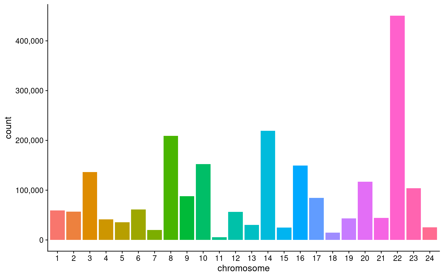
For the purpose of mapping the F₂ sample sequences to the genomes of their parental strains, we selected only biallelic SNPs that were homozygous-divergent in the F₀ generation (i.e. homozygous reference allele in Cab and homozygous alternative allele in Kaga or vice versa) and heterozygous in the F₁ generation. The number of SNPs that met these criteria per chromosome are set out in Figure 4.2. The strong homozygosity of Kaga on chr22 is likely responsible for the much greater number of loci on that chromosome that can be used for calling genoytpes in the F₂ generation, and highlights the importance of the parental strains being highly homozygous when used in experimental crosses such as this.

Code

# Load libraries

library(tidyverse)

# Get variables

## Debug

IN = "/hps/nobackup/birney/users/ian/somites/sites_files/F0_Cab_Kaga/hdrr/homo_divergent/F1_het_min_DP.txt"

df = readr::read_tsv(IN,
                     col_names = c("CHROM", "POS_1", "POS_2", "REF", "ALT", "F0_1_GT", "F0_2_GT"))

# Plot

df %>% 
  dplyr::count(CHROM) %>% 
  dplyr::mutate(CHROM = factor(CHROM, levels = sort(unique(CHROM)))) %>% 
  ggplot() +
  geom_col(aes(CHROM, n, fill = CHROM)) +
  guides(fill = "none") +
  cowplot::theme_cowplot() +
  xlab("chromosome") + 
  ylab("count") +
  scale_y_continuous(labels = scales::comma)

Figure 4.2: Number of SNPs per chromosome that were homozygous-divergent in the F₀ Cab and Kaga generations, and heterozygous in the F₁ generation. Code adapted from rule plot_SNP_counts_per_chr in https://github.com/brettellebi/somites/blob/master/workflow/rules/04_trio_homozygosity.smk.