2  Phenotypes of interest

2.1 Somite development period

Figure 2.1 shows the period data generated by pyBOAT for this study, for 100 illustrative F₂ samples over 300 minutes. The same data can be represented by boxplots as shown in Figure 2.2. We experimented with using the F₂ individuals’ mean period and period intercept as the phenotype of interest. The two measures are highly correlated (\(Pearson's~r =\) 0.84, \(p\) < 2.2 x 10^-16), so after displaying the distributions for both measures in Figure 2.4, we only show the analysis of period intercept, as it would appear to potentially be more robust to the changes in slope that can be observed in Figure 2.1.

Figure 2.1: PyBOAT results for 100 illustrative F₂ samples, showing the period length in minutes over the course of 300 minutes. Period tends to increase over time, meaning that as the embryo develops, each successive somite takes longer to form. Figure generated by Ali Seleit.

Figure 2.2: Period measurements for 70 F₂ individuals displayed as boxplots with each individual’s median and interquartile range. Figure generated by Ali Seleit.

2.2 Unsegmented presomitic mesoderm area (PSM)

In the proceeding analyses, we also included a second phenotype of interest: the total area of the unsegmented tissue at the stage where 10-11 somites had been formed (PSM area). As the measure is simply based on the total number of pixels covered by the embryo object, we considered it to be potentially more robust than the period measurements, and therefore included it as a type of positive control for the genetic association analyses on the period phenotype. The measurements for PSM area comparing F₀ Cab and Kaga strains are shown in Figure 2.3.

Figure 2.3: Measurements of unsegmented PSM area in pixels for the F₀ individuals from the Cab strain (\(N = 19\)) and Kaga strain (\(N = 10\)). Kaga tends to have a smaller PSM than Cab. Figure generated by Ali Seleit.

2.3 Comparisons between F₀, F₁ and F₂ generations

Figure 2.4 shows the distributions of the period intercept and unsegmented PSM area phenotypes across the F₀, F₁ and F₂ generations. In relation to the period intercept phenotype, only the Cab strain in shown for F₀ because only the Cab strain carries the reporter gene, which prohibited the collection of data for Kaga using this pyBOAT method. However, from previous bright field image analyses (which did not require the reporter), we determined that the Kaga strain has a lower (i.e. faster) period than Cab by around 10 minutes (see Figure 1.1). Given these differences, the F₁ generation shows the expected intermediate median between the Cab and Kaga F₀ strains. We also expected to observe that the F₂ generation has a similar median to the F₁ generation, but with a wider variance that spans across the extremes of the two F₀ parental strains.

Instead, we observed that the F₂ generation has a median that is slightly slower than the median of the slower-period F₀ Cab strain. These observations were unlikely to have been caused by technical issues. A possible biological explanation is that there are more genetic combinations that slow down the clock rather than speed it up (Sanchez et al. 2022; Schröter and Oates 2010). This phenomenon could be exacerbated by the Cab and Kaga strains originating from different Japanese medaka populations (southern and northern respectively), which are understood to be at the point of speciation (Katsumura et al. 2019). This slower period may therefore be driven by a biological incompatibility between their genomes in cases where they do not have a complete chromosome from each parent (as the F₁ generation does). We nevertheless proceeded with the genetic analysis with a view to potentially discovering the reason for this unusual distribution.

Code

IN_F01 = here::here("data/F0_F1_period.xlsx")
IN_F2 = here::here("config/phenos_with_reporter_genoandpheno.csv")

########################
# Plotting parameters
########################

# Intercept
intercept_pal = c("#8D99AE", "#2b2d42")

# Mean
mean_pal = c("#177E89", "#084C61")

# PSM
unsegmented_psm_area_pal = c("#D9D0DE", "#401F3E")

# Get lighter/darker functions

devtools::source_gist("c5015ee666cdf8d9f7e25fa3c8063c99")

########################
# Read in file
########################

df_f2 = readr::read_delim(IN_F2, delim = ";") %>% 
  # add `GEN` column
  dplyr::mutate(GEN = "F2")


# Read in F0 and F1 data
df_f01 = readxl::read_xlsx(IN_F01) %>% 
  dplyr::mutate(sample = fish) %>% 
  dplyr::mutate(GEN = dplyr::case_when(str_detect(fish, "^C") ~ "F0",
                                       str_detect(fish, "^K") ~ "F1"))

# Bind two data frames
df_all = dplyr::bind_rows(df_f01, df_f2) %>% 
  # factorise Microscope
  dplyr::mutate(Microscope = factor(Microscope, levels = c("AU", "DB")))

########################
# Kruskal-Wallis test
########################

## Difference between microscopes in period intercept for F2s

kw_df = df_all %>% 
  # take only F2 individuals
  dplyr::filter(GEN == "F2") %>% 
  # pivot longer to put phenotypes values in one column
  tidyr::pivot_longer(cols = c(mean, intercept, unsegmented_psm_area),
                      names_to = "phenotype",
                      values_to = "value") %>% 
  dplyr::group_by(phenotype) %>% 
  tidyr::nest() %>%
  dplyr::mutate(model = purrr::map(data,
                                   ~kruskal.test(x = .$value, g = .$Microscope))) %>%
  dplyr::select(-data) %>% 
  dplyr::mutate(model_tidy = purrr::map(model, broom::tidy)) %>%
  tidyr::unnest(model_tidy) %>% 
  rstatix::add_significance(p.col = "p.value") %>% 
  # remove model
  dplyr::select(-model) %>% 
  # reduce to 3 digits
  dplyr::mutate(p.value = signif(p.value, digits = 3)) %>% 
  # paste p-value with significance
  dplyr::mutate(p_final = dplyr::case_when(p.value.signif == "ns" ~ paste("p =", p.value),
                                           TRUE ~ paste("p =", p.value, p.value.signif))) %>% 
  # add `Microscope` column with 'DB' so that the text maps there on the plots
  dplyr::mutate(Microscope = factor("DB", levels = c("AU", "DB")))

########################
# Plot
########################

########### Intercept

intercept_fig = df_all %>% 
  # remove NAs
  dplyr::filter(!is.na(Microscope)) %>% 
  ggplot(aes(GEN, intercept, fill = Microscope)) +
  geom_violin() + 
  geom_boxplot(width = 0.3) +
  ggbeeswarm::geom_beeswarm(aes(GEN, intercept, colour = Microscope), size = 0.4, alpha = 0.5) +
  facet_grid(cols = vars(Microscope)) + 
  scale_colour_manual(values = lighter(intercept_pal, amount = 50)) +
  scale_fill_manual(values = darker(intercept_pal, amount = 50)) +
  cowplot::theme_cowplot() +
  theme(strip.background.x = element_blank(),
        strip.text.x = element_text(face = "bold")) +
  xlab("generation") +
  ylab("period intercept (minutes)") +
  guides(fill = "none",
         colour = "none") +
  # add p-value
  geom_text(data = kw_df %>% 
              dplyr::filter(phenotype == "intercept"),
            aes(x = "F2", y = -Inf, label = p_final,
                vjust = -1
            ))

########### PSM

psm_fig = df_all %>% 
  # remove NAs
  dplyr::filter(!is.na(Microscope)) %>% 
  ggplot(aes(GEN, unsegmented_psm_area, fill = Microscope)) +
  geom_violin() + 
  geom_boxplot(width = 0.3) +
  ggbeeswarm::geom_beeswarm(aes(GEN, unsegmented_psm_area, colour = Microscope), size = 0.4, alpha = 0.5) +
  facet_grid(cols = vars(Microscope)) + 
  scale_colour_manual(values = lighter(unsegmented_psm_area_pal, amount = 50)) +
  scale_fill_manual(values = darker(unsegmented_psm_area_pal, amount = 50)) +
  cowplot::theme_cowplot() +
  theme(strip.background.x = element_blank(),
        strip.text.x = element_text(face = "bold")) +
  xlab("generation") +
  ylab("unsegmented PSM area (pixels)") +
  guides(fill = "none",
         colour = "none") +
  # add p-value
  geom_text(data = kw_df %>% 
              dplyr::filter(phenotype == "unsegmented_psm_area"),
            aes(x = "F2", y = -Inf, label = p_final,
                vjust = -1
            ))


period_final = cowplot::plot_grid(intercept_fig,
                                  psm_fig,
                                  align = "hv",
                                  nrow = 2,
                                  labels = c("A", "B"),
                                  label_size = 16)

period_final

Figure 2.4: Comparisons between the F₀, F₁ and F₂ generations for period intercept and unsegmented PSM area. As only the Cab strain contains the reporter gene, the F₀ only shows period intercept for Cab individuals (with the Kaga strain previously estimated to have a period of ~10 minutes slower than Cab). A: period intercept in minutes. B: unsegmented PSM area in pixels. \(P\)-values are derived from Kruskal-Wallis tests comparing the F₂ individuals across microscopes. For unsegmented PSM area, data was only collected for the F₂ generation. Code adapted from rule phenotype_plots in https://github.com/brettellebi/somites/blob/master/workflow/rules/08_extra.smk

Another important issue to note is that the F₂ individuals were imaged using different microscopes of the same model (Zeiss LSM 780) but with different temperature control units and incubator boxes, denoted as ‘AU’ and ‘DB’.¹ We noticed that there was a difference between the microscopes in their temperatures of 0.7-0.8°C, translating to a 4-minute difference in the F₂ means for the period intercept measure (Kruskal-Wallis = 177.97, \(p\) = 1.34 x 10^-40), and a 3.5-minute difference in the F₂ means for the period mean measure (Kruskal-Wallis = 141.79, \(p\) = 1.08 x 10^-32). This difference would need to be accounted for in the downstream analysis through either adjusting the phenotype prior to running the genetic association model, or by including microscope as a covariate in the model. For unsegmented PSM area, we did not find a significant difference between microscopes, so we determined that it was not necessary to control for microscope in the downstream analysis for this phenotype.

2.3.0.1 Inverse-normalisation

To resolve this difference between microscopes for the period intercept data, we elected to transform it for the F₂ generation by “inverse-normalising” the period intercept within each microscope (Figure 2.5), and used this transformed phenotype for the downstream analysis. Inverse-normalisation is a rank-based normalisation approach which involves replacing the values in the phenotype vector with their rank (where ties are averaged), then converting the ranks into a normal distribution with the quantile function (Wichura 1988). The inverse-normalisation function I used for this analysis is set out in the following R code:

invnorm = function(x) {
  res = rank(x)
  # The arbitrary 0.5 value is added to the denominator below 
  # to avoid `qnorm()` returning 'Inf' for the last-ranked value
  res = qnorm(res/(length(res)+0.5))
  return(res)
}

Code

# Set variables

## Debug
IN_F2 = here::here("config/phenos_with_reporter_genoandpheno.csv")
OUT_PNG = here::here("book/plots/phenotypes/invnorm_intercept.png")
OUT_PDF = here::here("book/plots/phenotypes/invnorm_intercept.pdf")

########################
# Plotting parameters
########################

# Intercept
intercept_pal = c("#8D99AE", "#2b2d42")

# Mean
mean_pal = c("#177E89", "#084C61")

# PSM
unsegmented_psm_area_pal = c("#D9D0DE", "#401F3E")

# Get lighter/darker functions

devtools::source_gist("c5015ee666cdf8d9f7e25fa3c8063c99")

########################
# Read in file
########################

df_f2 = readr::read_delim(IN_F2, delim = ";") %>% 
  # add `GEN` column
  dplyr::mutate(GEN = "F2") %>% 
  # factorise Microscope
  dplyr::mutate(Microscope = factor(Microscope, levels = c("AU", "DB")))

# Get means per microscope
f2_means_notrans = df_f2 %>% 
  dplyr::filter(!is.na(Microscope)) %>% 
  dplyr::group_by(Microscope) %>% 
  dplyr::summarise(MEAN = mean(intercept, na.rm = T))


########################
# Plot
########################

########### Histogram raw

raw_fig = df_f2 %>% 
  # remove NAs
  dplyr::filter(!is.na(Microscope)) %>% 
  ggplot(aes(intercept)) +
  geom_histogram(aes(y = ..density.., fill = Microscope), bins = 40) +
  geom_density(aes(colour = Microscope)) +
  geom_vline(data = f2_means_notrans, aes(xintercept = MEAN)) +
  scale_fill_manual(values = intercept_pal) +
  scale_colour_manual(values = darker(intercept_pal,amount = 75)) +
  cowplot::theme_cowplot() + 
  facet_grid(rows = vars(GEN, Microscope)) +
  xlab('period intercept') + 
  guides(fill = "none", colour = "none") +
  labs(subtitle = "original data")

########### Histogram inverse-normalised

trans_df = df_f2 %>% 
  # inverse-normalise within microscope
  dplyr::group_by(Microscope) %>% 
  dplyr::mutate(intercept = invnorm(intercept)) %>% 
  dplyr::ungroup() %>% 
  # remove NAs
  dplyr::filter(!is.na(Microscope))

# Get means per microscope
f2_means_trans = trans_df %>% 
  dplyr::filter(!is.na(Microscope)) %>% 
  dplyr::group_by(Microscope) %>% 
  dplyr::summarise(MEAN = mean(intercept, na.rm = T))

trans_fig = trans_df %>% 
  # plot
  ggplot(aes(intercept)) +
  geom_histogram(aes(y = ..density.., fill = Microscope), bins = 40) +
  geom_density(aes(colour = Microscope)) +
  geom_vline(data = f2_means_trans, aes(xintercept = MEAN)) +
  scale_fill_manual(values = intercept_pal) +
  scale_colour_manual(values = darker(intercept_pal,amount = 75)) +
  cowplot::theme_cowplot() + 
  facet_grid(rows = vars(GEN, Microscope)) +
  xlab('period intercept (inverse-normalised)') + 
  guides(fill = "none", colour = "none") +
  labs(subtitle = "inverse-normalised within microscope")


########### Together

final = cowplot::plot_grid(raw_fig,
                                  trans_fig,
                                  align = "hv",
                                  nrow = 2,
                                  labels = c("A", "B"),
                                  label_size = 16)

final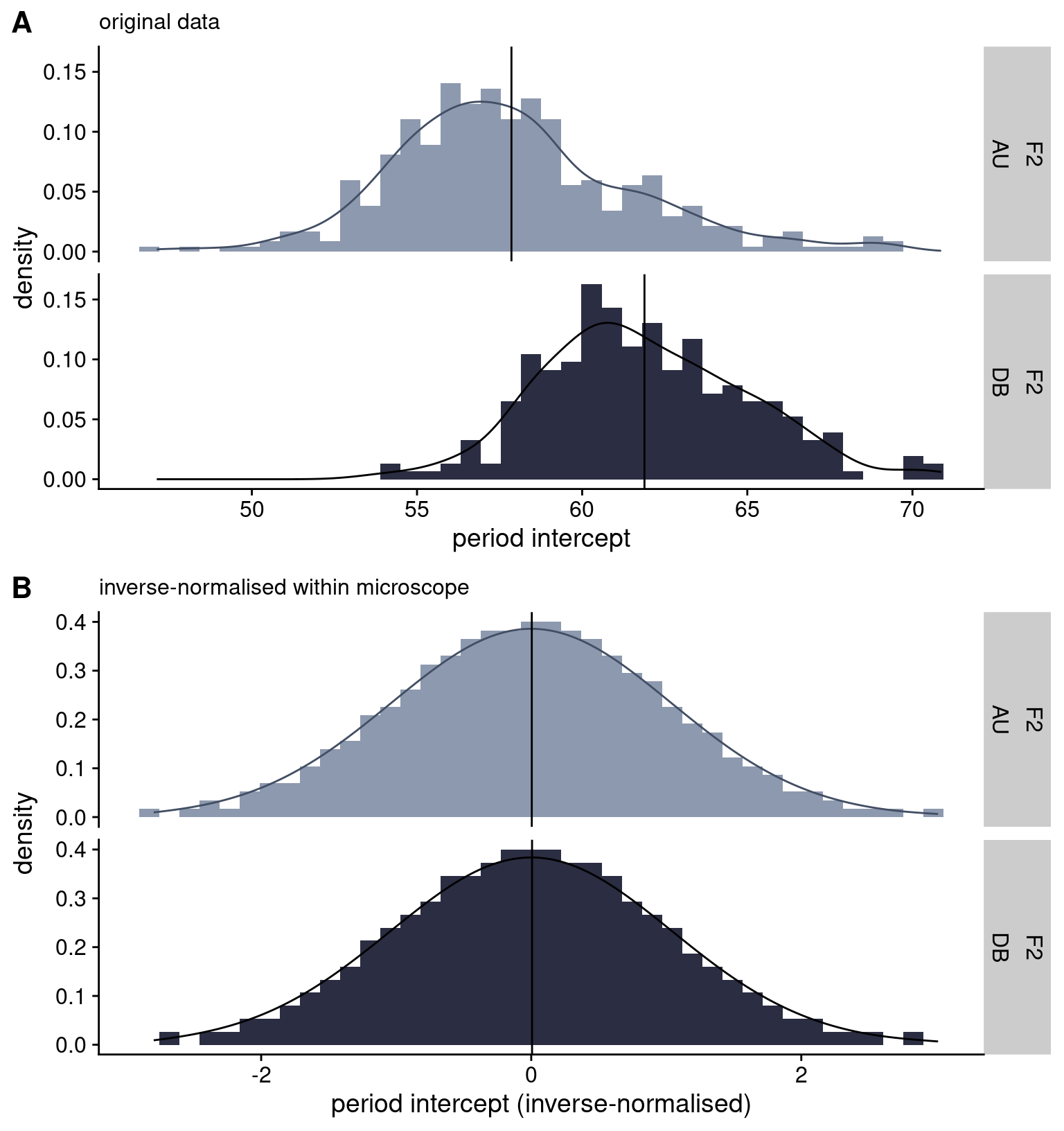

Figure 2.5: Comparison of the period intercept phenotype data for the F₂ generation before (A) and after (B) inverse-normalisation, with vertical lines marking the mean of each group. Code adapted from rule invnorm_intercept_plot in https://github.com/brettellebi/somites/blob/master/workflow/rules/08_extra.smk.

Katsumura, Takafumi, Shoji Oda, Hiroshi Mitani, and Hiroki Oota. 2019. “Medaka Population Genome Structure and Demographic History Described via Genotyping-by-Sequencing.” G3 Genes|Genomes|Genetics 9 (1): 217–28. https://doi.org/10.1534/g3.118.200779.

Sanchez, Paul Gerald Layague, Victoria Mochulska, Christian Mauffette Denis, Gregor Mönke, Takehito Tomita, Nobuko Tsuchida-Straeten, Yvonne Petersen, Katharina F. Sonnen, Paul François, and Alexander Aulehla. 2022. “Arnold Tongue Entrainment Reveals Dynamical Principles of the Embryonic Segmentation Clock.” bioRxiv. https://doi.org/10.1101/2021.10.20.465101.

Schröter, Christian, and Andrew C. Oates. 2010. “Segment Number and Axial Identity in a Segmentation Clock Period Mutant.” Current Biology 20 (14): 1254–58. https://doi.org/10.1016/j.cub.2010.05.071.

Wichura, Michael J. 1988. “Algorithm AS 241: The Percentage Points of the Normal Distribution.” Journal of the Royal Statistical Society. Series C (Applied Statistics) 37 (3): 477–84. https://doi.org/10.2307/2347330.

---

1. ‘AU’ for the Aulehla Lab microscope, and ‘DB’ for EMBL-Heidelberg’s Developmental Biology Unit microscope.