1 Load libraries

library(here)
library(tidyverse)
library(karyoploteR)
library(plotly)
library(circlize)
library(GGally)
library(viridis)

2 Snakemake pipeline to process VCF and extract data

https://github.com/brettellebi/mikk_genome/tree/master/code/snakemake/nucleotide_diversity

Steps

Filter MIKK panel VCF for non-sibling lines (N = 63).
Use VCFtools’s --window-pi to calculate nucleotide divergence in different-sized windows.
Use bcftools to extract MQ from INFO field.

3 Process data

Data location: /nfs/research/birney/users/ian/mikk_genome/nucleotide_divergence

3.1 Read in data

3.1.1 MIKK

# Set location of data
in_dir = "/nfs/research/birney/users/ian/mikk_genome/nucleotide_divergence/mikk/all"

in_files = list.files(in_dir, full.names = T)
dat_list = lapply(in_files, function(IN_FILE) {
  # Read in 
  readr::read_delim(IN_FILE,
                    delim = "\t",
                    col_types = c("ciiid")) %>% 
    # Remove MT
    dplyr::filter(CHROM != "MT") %>% 
    # Make CHR an integer
    dplyr::mutate(CHROM = as.integer(CHROM)) %>% 
    # Create middle of bin
    dplyr::mutate(BIN_MID = ((BIN_END - BIN_START - 1) / 2) + BIN_START )
})
names(dat_list) = basename(in_files) %>%
  str_remove(".windowed.pi")

3.1.2 Wild Kiyosu

# Set location of data
in_dir = "/nfs/research/birney/users/ian/mikk_genome/nucleotide_divergence/wild_kiyosu"

in_files = list.files(in_dir, full.names = T)
wk_list = lapply(in_files, function(IN_FILE) {
  # Read in 
  readr::read_delim(IN_FILE,
                    delim = "\t",
                    col_types = c("ciiid")) %>% 
    # Remove MT
    dplyr::filter(CHROM != "MT") %>% 
    # Make CHR an integer
    dplyr::mutate(CHROM = as.integer(CHROM)) %>% 
    # Create middle of bin
    dplyr::mutate(BIN_MID = ((BIN_END - BIN_START - 1) / 2) + BIN_START )
})
names(wk_list) = basename(in_files) %>%
  str_remove(".windowed.pi")

4 Karyoplot

4.1 Set up scaffold

med_chr_lens = read.table(here::here("data",
                                     "Oryzias_latipes.ASM223467v1.dna.toplevel.fa_chr_counts.txt"),
                          col.names = c("chr", "end"))
# Add start
med_chr_lens$start = 1
# Reorder
med_chr_lens = med_chr_lens %>% 
  dplyr::select(chr, start, end) %>% 
  # remove MT
  dplyr::filter(chr != "MT") %>% 
  # convert to numeric
  dplyr::mutate(chr = as.integer(chr)) %>% 
  # order
  dplyr::arrange(chr)

# Create custom genome 
med_genome = regioneR::toGRanges(med_chr_lens)

4.2 Plot

4.2.1 Compare effect of bin width on noise

# Test with ggplot
dat_list$`1000000` %>% 
  ggplot() +
    geom_line(aes(BIN_MID, PI)) +
    facet_grid(cols = vars(CHROM))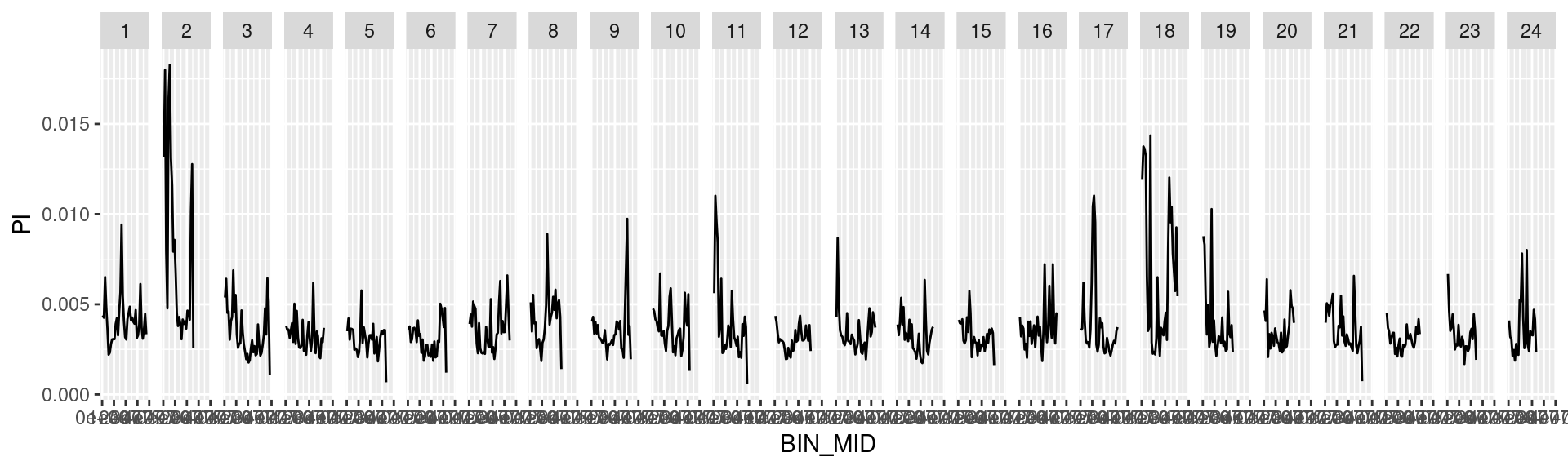

dat_list$`500000` %>% 
  ggplot() +
    geom_line(aes(BIN_MID, PI)) +
    facet_grid(cols = vars(CHROM))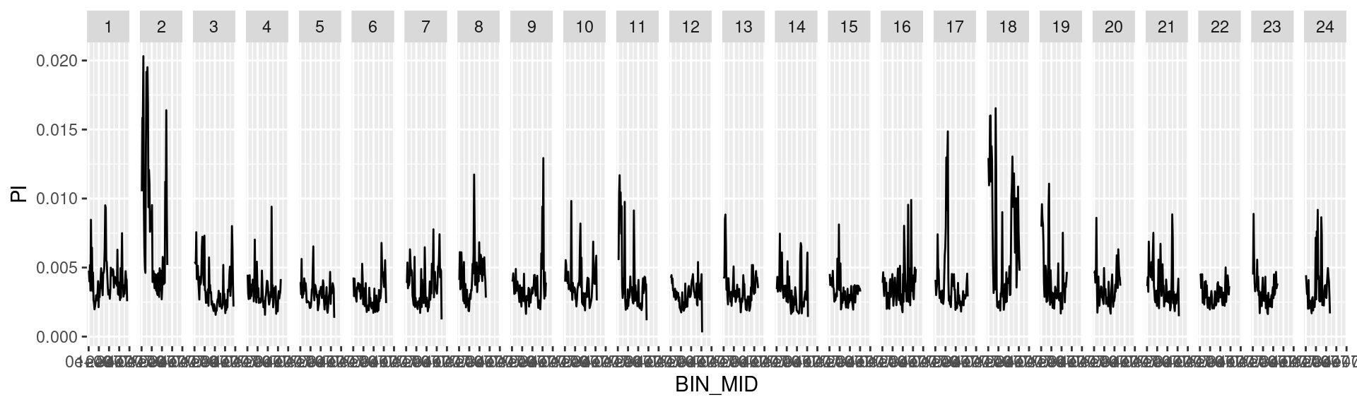

dat_list$`100000` %>% 
  ggplot() +
    geom_line(aes(BIN_MID, PI)) +
    facet_grid(cols = vars(CHROM))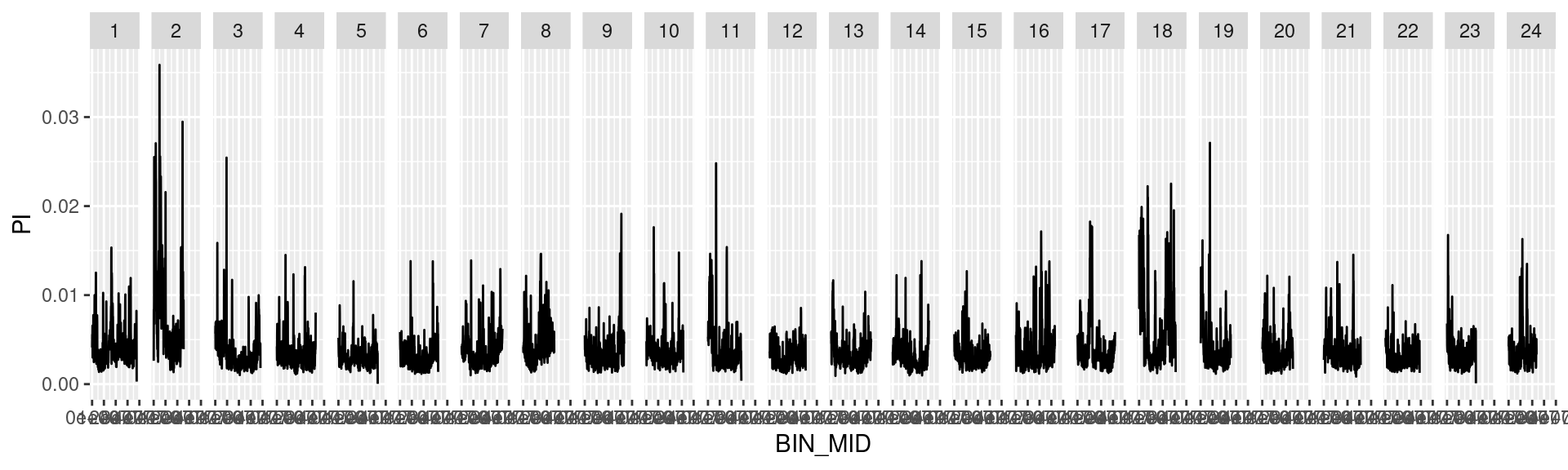

## Get max Y
round.choose <- function(x, roundTo, dir = 1) {
  if(dir == 1) {  ##ROUND UP
    x + (roundTo - x %% roundTo)
  } else {
    if(dir == 0) {  ##ROUND DOWN
      x - (x %% roundTo)
    }
  }
}
y_max = round.choose(max(dat_list$`1000000`$PI), 0.01, 1)

# set file name
file_name = paste("20210930_", "1Mb", ".png", sep = "")
file_out = here::here("docs/plots/nucleotide_diversity", file_name)

png(file=file_out,
    width=13000,
    height=1000,
    units = "px",
    res = 300)

# Plot ideogram
kp = karyoploteR::plotKaryotype(med_genome, plot.type = 5)

# Add base numbers 
karyoploteR::kpAddBaseNumbers(kp, tick.dist = 5000000, cex = 0.7)

# Set y-axis limits
karyoploteR::kpAxis(kp, ymin=0, ymax=y_max )

# Add lines
lwd = 1
karyoploteR::kpLines(kp,
                     chr = dat_list$`1000000`$CHROM,
                     x = dat_list$`1000000`$BIN_MID,
                     y = dat_list$`1000000`$PI,
                     ymax = y_max,
                     r0=0, r1 = 1,
                     lwd = lwd)



dev.off()

file_out = here::here("docs/plots/nucleotide_diversity/20210930_1Mb.png")
knitr::include_graphics(file_out)

5 Circos

5.1 Get repeats data

repeats_file = "/nfs/research/birney/users/ian/mikk_genome/repeats/medaka_hdrr_repeats.fixed.gff"

hdrr_reps = readr::read_delim(repeats_file,
                              delim = "\t",
                              col_names = F,
                              skip = 3,
                              comment = "",
                              quote = "") %>%
  # Remove empty V8 column
  dplyr::select(-X8) %>% 
  # Get class of repeat from third column
  dplyr::mutate(class = stringr::str_split(X3, pattern = "#", simplify = T)[, 1]) %>% 
  # Rename columns
  dplyr::rename(chr = X1, tool = X2, class_full = X3, start = X4, end = X5, percent = X6, strand = X7, info = X9)

# Find types of class other than "(GATCCA)n" types
class_types = unique(hdrr_reps$class[grep(")n", hdrr_reps$class, invert = T)])

hdrr_reps = hdrr_reps %>%
  # NA for blanks
  dplyr::mutate(class = dplyr::na_if(class, "")) %>%
  # "misc" for others in "(GATCCA)n" type classes
  dplyr::mutate(class = dplyr::if_else(!class %in% class_types, "Miscellaneous", class)) %>%
  # rename "Simple_repeat"
  dplyr::mutate(class = dplyr::recode(class, "Simple_repeat" = "Simple repeat")) %>% 
  # filter out NA in `chr` (formerly MT)
  dplyr::filter(!is.na(chr))

5.2 Calculate proportion of bin covered by repeats

5.2.1 Bin intevals

# Create GRanges object with bins
bin_length = "1000000"

bin_intervals = dat_list[[bin_length]] %>% 
  dplyr::select(CHROM, BIN_START, BIN_END) %>% 
  # split into list by chromosome
  split(., f = .$CHROM)

# Replace END pos of final bin for each chromsome with actual end pos
bin_intervals = lapply(1:length(bin_intervals), function(CHR){
  # Get end position for target chromosome
  end_pos = med_chr_lens %>% 
    dplyr::filter(chr == CHR) %>% 
    dplyr::pull(end)
  # Replace final bin end position
  out = bin_intervals[[CHR]]
  out$BIN_END[nrow(out)] = end_pos
  
  return(out)
}) %>% 
  dplyr::bind_rows()

# Convert to data frame
bin_intervals = as.data.frame(bin_intervals)

# Convert to GRanges
bin_ranges = regioneR::toGRanges(bin_intervals)

5.2.2 Repeats

# Convert `hdrr_reps` to GRanges
hdrr_ranges = GenomicRanges::makeGRangesFromDataFrame(hdrr_reps,
                                                      keep.extra.columns = T,
                                                      seqnames.field = "chr",
                                                      start.field = "start",
                                                      end.field = "end")

# Get non-overlapping regions
hdrr_covered = GenomicRanges::disjoin(hdrr_ranges)

5.2.3 Find quantity of repeats overlapping bins

overlaps = GenomicRanges::findOverlaps(bin_ranges, hdrr_covered)

# Split into list by bin
overlaps_list = lapply(unique(overlaps@from), function(BIN){
  out = list()
  # Get indexes of all repeat ranges overlapping the target BIN
  out[["hits"]] = overlaps[overlaps@from == BIN]@to
  # Extract those ranges from `hdrr_ranges`
  out[["range_hits"]] = hdrr_covered[out[["hits"]]]
    # Get number bases covered by each range
  out[["widths"]] = out[["range_hits"]] %>% 
    GenomicRanges::width(.) 
  # Get summed widths
  out[["summed"]] = out[["widths"]] %>% 
    # Get total bases covered in bin
    sum(.)
  
  return(out)
})
  
overlaps_vec = purrr::map(overlaps_list, function(BIN){
  BIN[["summed"]]
}) %>% 
  unlist(.)

# Add as column to `bin_intervals`
bin_intervals$REPEAT_COV = overlaps_vec

# Caclulate proportion
bin_intervals = bin_intervals %>%
  dplyr::mutate(REPEAT_PROP = REPEAT_COV / (BIN_END - BIN_START + 1))

5.3 Read in mapping quality scores

in_file = "/nfs/research/birney/users/ian/mikk_genome/mapping_quality/mapping_quality.csv"

mq_df = readr::read_csv(in_file,
                        col_names = c("CHROM", "POS", "MQ"),
                        col_types = c("cid")) %>% 
  # remove 'MT'
  dplyr::filter(!CHROM == "MT") %>% 
  # make CHROM integer
  dplyr::mutate(CHROM = as.integer(CHROM))

# Bin and get means
mq_list = mq_df %>% 
  split(., f = .$CHROM)

# Bin into 1 Mb intervals
binned_mq_list = purrr::map(mq_list, function(CHR){
  # Set intervals
  intervals = seq(1, max(CHR$POS), by = 1000000)
  # add final length
  if (max(intervals) != max(CHR$POS)) {
    intervals = c(intervals, max(CHR$POS))
  }
  # bin
  CHR = CHR %>% 
    dplyr::mutate(BIN = cut(POS,
                            breaks = intervals,
                            labels = F,
                            include.lowest = T))
})

# calculate mean MQ within each bin
mean_mq = purrr::map(binned_mq_list, function(CHR){
  CHR %>% 
    # replace Inf with NA
    dplyr::mutate(MQ = dplyr::na_if(MQ, Inf)) %>% 
    # Group by BIN
    dplyr::group_by(BIN) %>% 
    # Calculate mean MQ within each bin
    dplyr::summarise(MEAN_MQ = mean(MQ, na.rm = T))
}) %>% 
  # bind into single data frame
  dplyr::bind_rows(.id = "CHR")

## Warning: One or more parsing issues, see `problems()` for details

5.4 Bind data frames

# Bind data frames
pi_repeat_df = cbind(dat_list$`1000000`,
                     PI_WK = wk_list[["1000000"]]$PI,
                     REPEAT_PROP = bin_intervals$REPEAT_PROP,
                     MEAN_MQ = mean_mq$MEAN_MQ)

5.5 Pairs plot

pairs_plot = GGally::ggpairs(pi_repeat_df, columns = c(5, 7, 8, 9),
                             lower = list(continuous = wrap("points", alpha = 0.2, size = 0.5),
                                          combo = wrap("dot_no_facet", alpha = 0.4)))

plotly::ggplotly(pairs_plot)

## Warning: Can only have one: highlight

## Warning: Can only have one: highlight

## Warning: Can only have one: highlight

5.6 Circos

5.6.1 1 Mb

5.6.1.1 Rearrange data frames

df_circos_1Mb = pi_repeat_df
# take `BIN_END` from `bin_intervals` with chromosome end number for final bin
df_circos_1Mb$BIN_END = bin_intervals$BIN_END

5.6.1.2 Plot

out_plot = here::here("docs/plots/nucleotide_diversity", "20211001_circos_1Mb.png")

png(out_plot,
    width = 20,
    height = 20,
    units = "cm",
    res = 500)

# Set parameters
## Decrease cell padding from default c(0.02, 1.00, 0.02, 1.00)
circos.par(cell.padding = c(0, 0, 0, 0),
           track.margin = c(0, 0),
           gap.degree = c(rep(1, nrow(med_chr_lens) - 1), 6))
# Initialize plot
circos.initializeWithIdeogram(med_chr_lens,
                              plotType = c("axis", "labels"),
                              major.by = 1e7,
                              axis.labels.cex = 0.25*par("cex"))

# Add MIKK Pi line
circos.genomicTrack(df_circos_1Mb,
    panel.fun = function(region, value, ...){
  circos.genomicLines(region,
                      value[[2]],
                      col = "#49A379",
                      area = T,
                      border = karyoploteR::darker("#49A379"))
    },
    track.height = 0.1,
    bg.border = NA,
    ylim = c(0, 0.021))

circos.yaxis(side = "right",
           at = c(.01, .02),
           labels.cex = 0.25*par("cex"),
           tick.length = 2
           )

circos.text(0, 0.01,
        labels = expression(paste("MIKK (", pi, ")", sep = "")),
        sector.index = "1",
        facing = "clockwise",
        adj = c(.5, 0),
        cex = 0.4*par("cex"))

## Note: 1 point is out of plotting region in sector '1', track '2'.

# Add wild Kiyosu line
circos.genomicTrack(df_circos_1Mb,
    panel.fun = function(region, value, ...){
  circos.genomicLines(region,
                      value[[4]],
                      col = "#7A306C",
                      area = T,
                      border = karyoploteR::darker("#8A4F7D"))
    },
    track.height = 0.1,
    bg.border = NA,
    ylim = c(0, 0.021))

circos.yaxis(side = "right",
           at = c(.01, .02),
           labels.cex = 0.25*par("cex"),
           tick.length = 2
           )

circos.text(0, 0.01,
        labels = expression(paste("Wild\nKiyosu (", pi, ")", sep = "")),
        sector.index = "1",
        facing = "clockwise",
        adj = c(.5, 0),
        cex = 0.4*par("cex"))

## Note: 1 point is out of plotting region in sector '1', track '3'.

# Add repeat content
circos.genomicTrack(df_circos_1Mb,
  panel.fun = function(region, value, ...) {
    circos.genomicLines(region,
                        value[[5]],
                        type = "h",
                        col = "#0C1B33",
                        cex = 0.05,
                        baseline = 0)
  },
  track.height = 0.1,
  ylim = c(0,0.5),
  bg.border = NA)

circos.yaxis(side = "right",
           at = c(0, .5, 1),
           labels.cex = 0.25*par("cex"),
           tick.length = 5
           )

circos.text(0, 0.25,
        labels = "Repeat\ncontent",
        sector.index = "1",
        facing = "clockwise",
        adj = c(.5, 0),
        cex = 0.4*par("cex"))

## Note: 1 point is out of plotting region in sector '1', track '4'.

# Add mean mapping quality
circos.genomicTrack(df_circos_1Mb,
  panel.fun = function(region, value, ...) {
    circos.genomicLines(region,
                        value[[6]],
                        type = "h",
                        col = "#FF6978",
                        cex = 0.05,
                        baseline = 20)
  },
  track.height = 0.1,
  ylim = c(20,65),
  bg.border = NA)

circos.yaxis(side = "right",
           at = c(20, 50),
           labels.cex = 0.25*par("cex"),
           tick.length = 5
           )

circos.text(0, 40,
        labels = "Mean MQ",
        sector.index = "1",
        facing = "clockwise",
        adj = c(.5, 0),
        cex = 0.4*par("cex"))

## Note: 1 point is out of plotting region in sector '1', track '5'.

# Add baseline
#circos.xaxis(h = "bottom",
#             labels = F,
#             major.tick = F)

# Print label in center
text(0, 0, "Nucleotide diversity in\nMIKK and wild Kiyosu medaka,\nrepeat content,\nand mapping quality\nin 1 Mb windows")

circos.clear()

dev.off()

## png 
##   2

knitr::include_graphics(out_plot)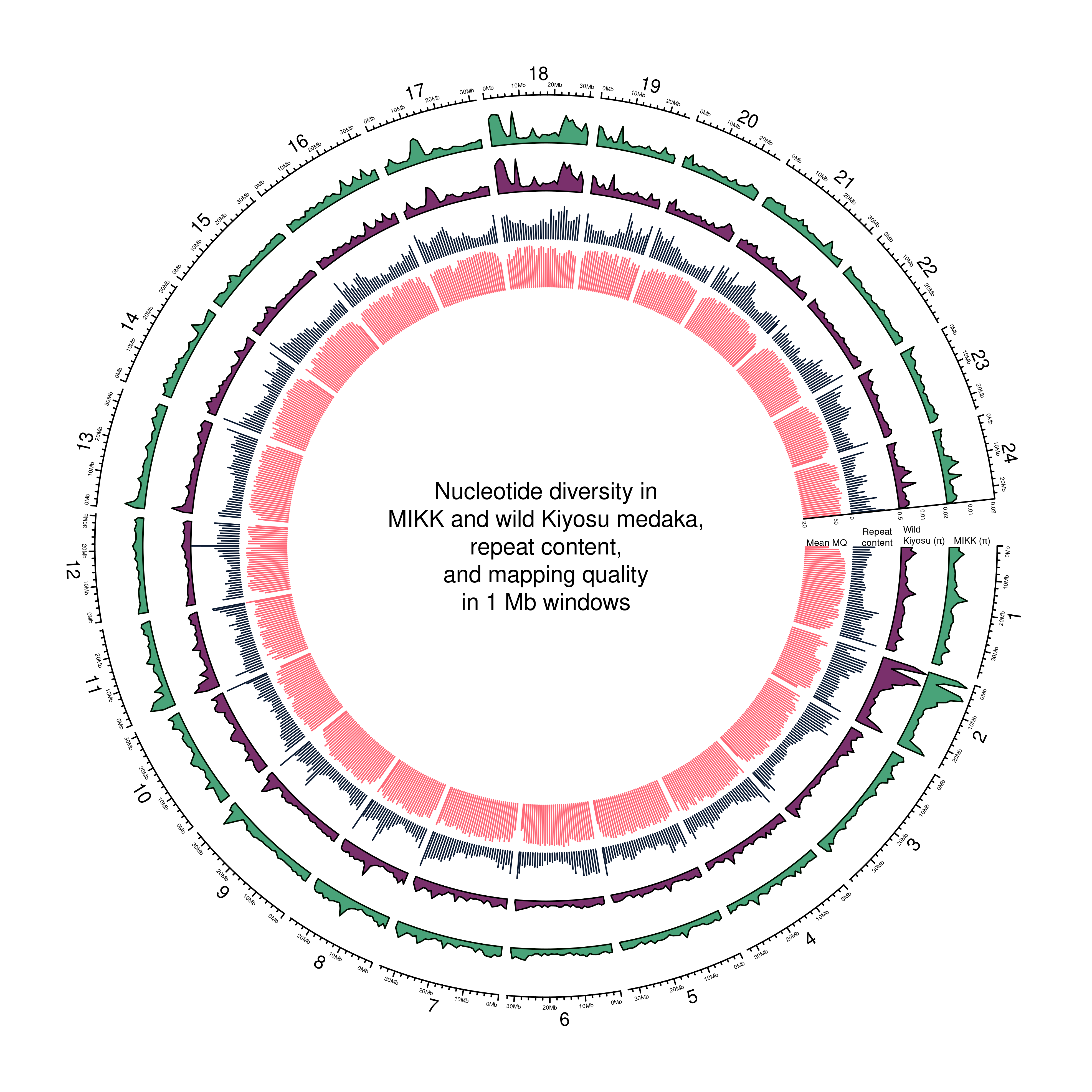

5.6.2 500 Kb

5.6.2.1 Create data frame

5.6.2.1.1 Repeats

# Create GRanges object with bins
bin_length = "500000"

bin_intervals_500 = dat_list[[bin_length]] %>% 
  dplyr::select(CHROM, BIN_START, BIN_END) %>% 
  # split into list by chromosome
  split(., f = .$CHROM)

# Replace END pos of final bin for each chromsome with actual end pos
bin_intervals_500 = lapply(1:length(bin_intervals_500), function(CHR){
  # Get end position for target chromosome
  end_pos = med_chr_lens %>% 
    dplyr::filter(chr == CHR) %>% 
    dplyr::pull(end)
  # Replace final bin end position
  out = bin_intervals_500[[CHR]]
  out$BIN_END[nrow(out)] = end_pos
  
  return(out)
}) %>% 
  dplyr::bind_rows()

# Convert to data frame
bin_intervals_500 = as.data.frame(bin_intervals_500)

# Convert to GRanges
bin_ranges = regioneR::toGRanges(bin_intervals_500)
  
overlaps = GenomicRanges::findOverlaps(bin_ranges, hdrr_covered)

# Split into list by bin
overlaps_list = lapply(unique(overlaps@from), function(BIN){
  out = list()
  # Get indexes of all repeat ranges overlapping the target BIN
  out[["hits"]] = overlaps[overlaps@from == BIN]@to
  # Extract those ranges from `hdrr_ranges`
  out[["range_hits"]] = hdrr_covered[out[["hits"]]]
    # Get number bases covered by each range
  out[["widths"]] = out[["range_hits"]] %>% 
    GenomicRanges::width(.) 
  # Get summed widths
  out[["summed"]] = out[["widths"]] %>% 
    # Get total bases covered in bin
    sum(.)
  
  return(out)
})
  
overlaps_vec = purrr::map(overlaps_list, function(BIN){
  BIN[["summed"]]
}) %>% 
  unlist(.)

# Add as column to `bin_intervals_500`
bin_intervals_500$REPEAT_COV = overlaps_vec

# Caclulate proportion
bin_intervals_500 = bin_intervals_500 %>%
  dplyr::mutate(REPEAT_PROP = REPEAT_COV / (BIN_END - BIN_START + 1))

5.6.2.1.2 MQ

# Bin into 1 Mb intervals
binned_mq_list_500 = purrr::map(mq_list, function(CHR){
  # Set intervals
  intervals = seq(1, max(CHR$POS), by = 500000)
  # add final length
  if (max(intervals) != max(CHR$POS)) {
    intervals = c(intervals, max(CHR$POS))
  }
  # bin
  CHR = CHR %>% 
    dplyr::mutate(BIN = cut(POS,
                            breaks = intervals,
                            labels = F,
                            include.lowest = T))
})

# calculate mean MQ within each bin
mean_mq_500 = purrr::map(binned_mq_list_500, function(CHR){
  CHR %>% 
    # replace Inf with NA
    dplyr::mutate(MQ = dplyr::na_if(MQ, Inf)) %>% 
    # Group by BIN
    dplyr::group_by(BIN) %>% 
    # Calculate mean MQ within each bin
    dplyr::summarise(MEAN_MQ = mean(MQ, na.rm = T))
}) %>% 
  # bind into single data frame
  dplyr::bind_rows(.id = "CHR")

5.6.2.1.3 Final

df_circos_500kb = cbind(dat_list$`500000`,
                        PI_WK = wk_list[["500000"]]$PI,
                        REPEAT_PROP = bin_intervals_500$REPEAT_PROP,
                        MEAN_MQ = mean_mq_500$MEAN_MQ)
# Add bin ends at the end of each chromosome to match real chromosome ends
df_circos_500kb$BIN_END = bin_intervals_500$BIN_END

out_plot = here::here("docs/plots/nucleotide_diversity/20211001_circos_500kb.png")

png(out_plot,
    width = 20,
    height = 20,
    units = "cm",
    res = 500)

# Set parameters
## Decrease cell padding from default c(0.02, 1.00, 0.02, 1.00)
circos.par(cell.padding = c(0, 0, 0, 0),
           track.margin = c(0, 0),
           gap.degree = c(rep(1, nrow(med_chr_lens) - 1), 6))
# Initialize plot
circos.initializeWithIdeogram(med_chr_lens,
                              plotType = c("axis", "labels"),
                              major.by = 1e7,
                              axis.labels.cex = 0.25*par("cex"))

# Add MIKK Pi line
circos.genomicTrack(df_circos_500kb,
    panel.fun = function(region, value, ...){
  circos.genomicLines(region,
                      value[[2]],
                      col = "#49A379",
                      area = T,
                      border = karyoploteR::darker("#49A379"))
    },
    track.height = 0.1,
    bg.border = NA,
    ylim = c(0, 0.023))

circos.yaxis(side = "right",
           at = c(.01, .02),
           labels.cex = 0.25*par("cex"),
           tick.length = 2
           )

circos.text(0, 0.01,
        labels = expression(paste("MIKK (", pi, ")", sep = "")),
        sector.index = "1",
        facing = "clockwise",
        adj = c(.5, 0),
        cex = 0.4*par("cex"))

## Note: 1 point is out of plotting region in sector '1', track '2'.

# Add wild Kiyosu line
circos.genomicTrack(df_circos_500kb,
    panel.fun = function(region, value, ...){
  circos.genomicLines(region,
                      value[[4]],
                      col = "#7A306C",
                      area = T,
                      border = karyoploteR::darker("#8A4F7D"))
    },
    track.height = 0.1,
    bg.border = NA,
    ylim = c(0, 0.023))

circos.yaxis(side = "right",
           at = c(.01, .02),
           labels.cex = 0.25*par("cex"),
           tick.length = 2
           )

circos.text(0, 0.01,
        labels = expression(paste("Wild\nKiyosu (", pi, ")", sep = "")),
        sector.index = "1",
        facing = "clockwise",
        adj = c(.5, 0),
        cex = 0.4*par("cex"))

## Note: 1 point is out of plotting region in sector '1', track '3'.

# Add repeat content
circos.genomicTrack(df_circos_500kb,
  panel.fun = function(region, value, ...) {
    circos.genomicLines(region,
                        value[[5]],
                        type = "h",
                        col = "#0C1B33",
                        lwd = 0.4,
                        cex = 0.05,
                        baseline = 0)
  },
  track.height = 0.1,
  ylim = c(0,0.65),
  bg.border = NA)

circos.yaxis(side = "right",
           at = c(0, .5, 1),
           labels.cex = 0.25*par("cex"),
           tick.length = 5
           )

circos.text(0, 0.325,
        labels = "Repeat\ncontent",
        sector.index = "1",
        facing = "clockwise",
        adj = c(.5, 0),
        cex = 0.4*par("cex"))

## Note: 1 point is out of plotting region in sector '1', track '4'.

# Add mean mapping quality
circos.genomicTrack(df_circos_500kb,
  panel.fun = function(region, value, ...) {
    circos.genomicLines(region,
                        value[[6]],
                        type = "h",
                        col = "#FF6978",
                        lwd = 0.4,
                        cex = 0.05,
                        baseline = 20)
  },
  track.height = 0.07,
  ylim = c(20,65),
  bg.border = NA)

circos.yaxis(side = "right",
           at = c(20, 50),
           labels.cex = 0.25*par("cex"),
           tick.length = 5
           )

circos.text(0, 40,
        labels = "Mean MQ",
        sector.index = "1",
        facing = "clockwise",
        adj = c(.5, 0),
        cex = 0.4*par("cex"))

## Note: 1 point is out of plotting region in sector '1', track '5'.

# Print label in center
text(0, 0, "Nucleotide diversity in\nMIKK and wild Kiyosu medaka,\nwith repeat content\nand mapping quality\nin 500 kb windows")

circos.clear()

dev.off()

## png 
##   2

knitr::include_graphics(out_plot)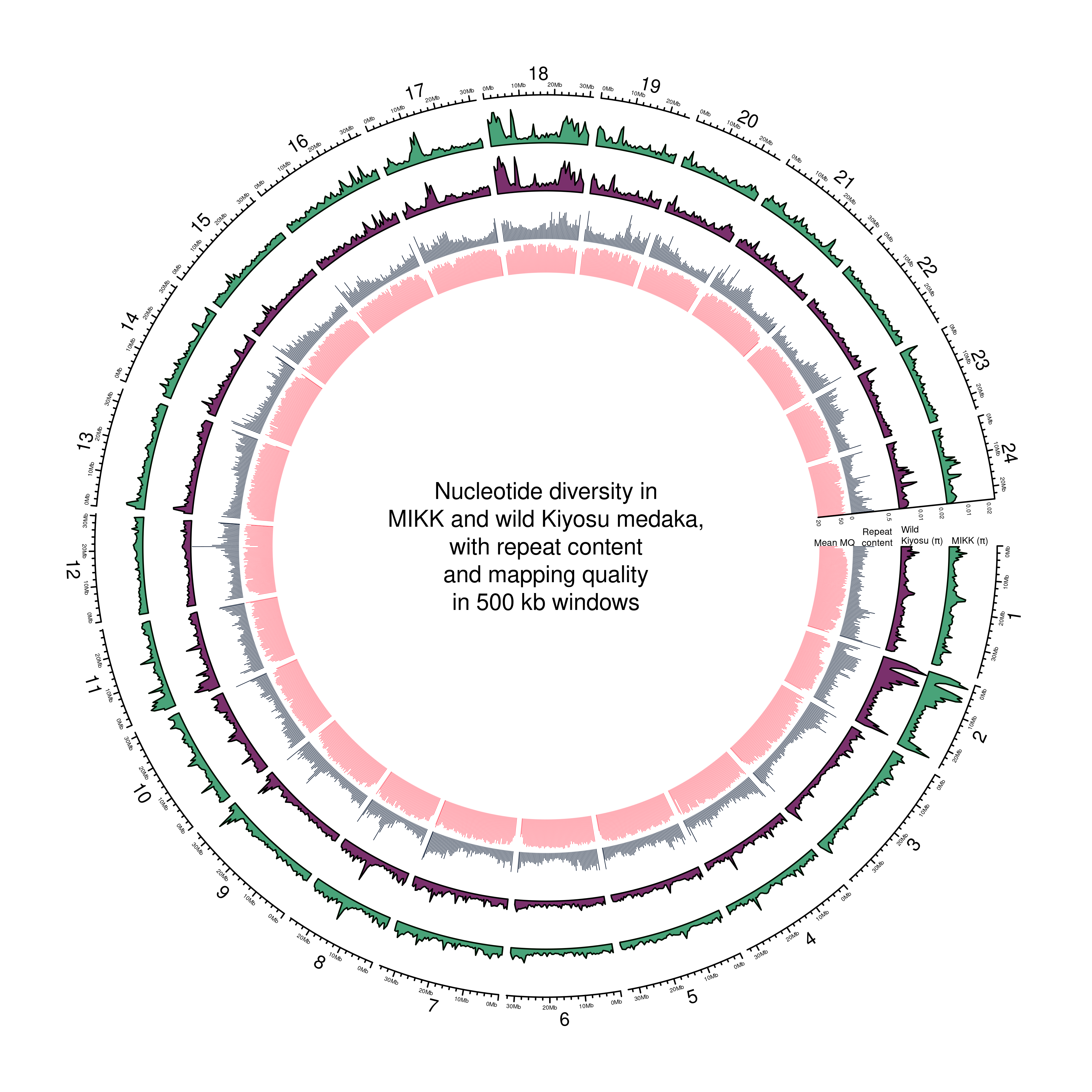

5.6.3 Mean and median Pi

5.6.3.1 63 MIKK samples v 7 wild Kiyosu

# MIKK 
mean(df_circos_500kb$PI)

## [1] 0.003829434

median(df_circos_500kb$PI)

## [1] 0.00329243

# Wild median Pi
mean(df_circos_500kb$PI_WK)

## [1] 0.003685076

median(df_circos_500kb$PI_WK)

## [1] 0.003102805

5.6.3.2 7 MIKK samples v 7 wild Kiyosu

# Read in data
mikk_7 = readr::read_delim("/nfs/research/birney/users/ian/mikk_genome/nucleotide_divergence/mikk/random/500.windowed.pi",
                  delim = "\t",
                  col_types = c("ciiid")) %>% 
  # Remove MT
  dplyr::filter(CHROM != "MT") %>% 
  # Make CHR an integer
  dplyr::mutate(CHROM = as.integer(CHROM)) %>% 
  # Create middle of bin
  dplyr::mutate(BIN_MID = ((BIN_END - BIN_START - 1) / 2) + BIN_START )

# Mean
mean(mikk_7$PI)

## [1] 0.003748531

median(mikk_7$PI)

## [1] 0.003197675

6 Per-individual

6.1 Read in data

6.1.1 MIKK

# Set location of data
in_dir = "/nfs/research/birney/users/ian/mikk_genome/nucleotide_divergence/mikk/per_sample"

in_files = list.files(in_dir, full.names = T)
mikk_list = lapply(in_files, function(IN_FILE) {
  # Read in 
  readr::read_delim(IN_FILE,
                    delim = "\t",
                    col_types = c("ciiid")) %>% 
    # Remove MT
    dplyr::filter(CHROM != "MT") %>% 
    # Make CHR an integer
    dplyr::mutate(CHROM = as.integer(CHROM)) %>% 
    # Create middle of bin
    dplyr::mutate(BIN_MID = ((BIN_END - BIN_START - 1) / 2) + BIN_START )
})
names(mikk_list) = basename(in_files) %>%
  str_remove(".windowed.pi")

# reorder
ordered_lines = tibble::tibble("LINE" = names(mikk_list)) %>% 
  tidyr::separate(col = LINE, into = c("LINE", "SIB", "EXTRA"), sep = "_") %>% 
  dplyr::mutate(LINE = as.integer(LINE)) %>% 
  dplyr::arrange(LINE) %>% 
  tidyr::unite(col = "ORIGINAL", sep = "_", na.rm = T) %>% 
  dplyr::pull()

## Warning: Expected 3 pieces. Missing pieces filled with `NA` in 62 rows [1, 2, 3, 4, 5, 6, 7, 8, 9, 10, 11, 12, 13, 15, 16,
## 17, 18, 19, 20, 21, ...].

mikk_list = mikk_list[order(match(names(mikk_list), ordered_lines))]

# Bind rows
mikk_df = mikk_list %>% 
  dplyr::bind_rows(.id = "LINE") %>% 
  # factor LINE to order
  dplyr::mutate(LINE = factor(LINE, levels = names(mikk_list)))

6.1.2 Wild

# Set location of data
in_dir = "/nfs/research/birney/users/ian/mikk_genome/nucleotide_divergence/wild/per_sample"

in_files = list.files(in_dir, full.names = T)
wild_list = lapply(in_files, function(IN_FILE) {
  # Read in 
  readr::read_delim(IN_FILE,
                    delim = "\t",
                    col_types = c("ciiid")) %>% 
    # Remove MT
    dplyr::filter(CHROM != "MT") %>% 
    # Make CHR an integer
    dplyr::mutate(CHROM = as.integer(CHROM)) %>% 
    # Create middle of bin
    dplyr::mutate(BIN_MID = ((BIN_END - BIN_START - 1) / 2) + BIN_START )
})
names(wild_list) = basename(in_files) %>%
  str_remove(".windowed.pi")

# Bind rows
wild_df = wild_list %>% 
  dplyr::bind_rows(.id = "LINE")

6.1.3 Combine

pi_df = list("MIKK" = mikk_df,
             "WILD" = wild_df) %>% 
  dplyr::bind_rows(.id = "POPULATION")

6.1.4 Boxplot

# Create palette
pal = c("#49A379", "#8A4F7D")
names(pal) = c("MIKK", "WILD")

mikk_wild_boxplot_no_filter = pi_df %>% 
  ggplot() +
    geom_violin(aes(POPULATION, log10(PI), colour = POPULATION, fill = POPULATION)) +
    geom_boxplot(aes(POPULATION, log10(PI), colour = POPULATION, fill = POPULATION), width = 0.1) +
    theme_bw() +
    scale_fill_manual(name = "Population", values = pal) +
    scale_colour_manual(name = "Population", values = darker(pal, 80)) +
    ylab(expression(paste(log[10], "(", pi, ")", sep = ""))) +
    ggtitle("Nucleotide diversity in 500 kb bins (MAPQ >= 50)")

mikk_wild_boxplot_no_filter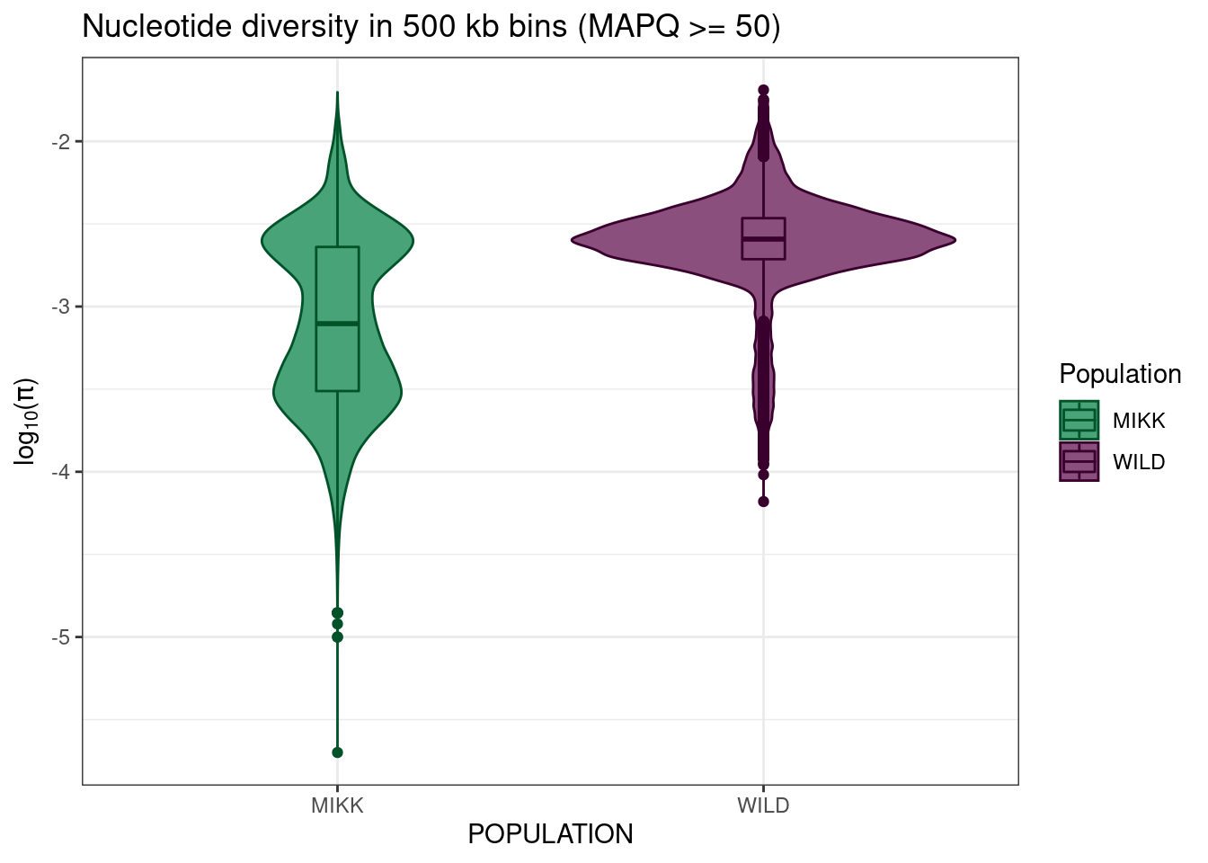

ggsave(here::here("docs/plots/nucleotide_diversity/20211006_mikk_wild_boxplot_no_filter.png"),
       plot = mikk_wild_boxplot_no_filter,
       device = "png",
       width = 8,
       height = 6,
       units = "in",
       dpi = 400)

6.1.5 All chromosomes

purrr::map(1:24, function(CHR){
    # Create plot
    plot_df = mikk_df %>% 
      # Filter for target CHROM
      dplyr::filter(CHROM == CHR) %>% 
      # Create Mb column
      dplyr::mutate(Mb = (BIN_START - 1) / 1e6)
    out_plot = plot_df %>% 
      ggplot() +
        geom_col(aes(Mb, PI, fill = PI)) +
        facet_grid(rows = vars(LINE), cols = vars(CHROM)) +
        theme_bw() +
        theme(text = element_text(size = 5)) +
        ylim(c(0, max(mikk_df$PI))) +
        xlab("500 kb window start position (Mb)") +
        ylab(expression(paste("Nucleotide diversity (", pi, ")", sep = ""))) +
        ggtitle(paste("Chromosome ", CHR, sep = "")) +
        scale_fill_viridis(name = expression(pi), limits = c(0,max(mikk_df$PI)))
        
    
    # Adjust width dimensions of plot based on length of chromosome
    w_dim = mikk_df %>% 
      dplyr::filter(CHROM == CHR) %>% 
      dplyr::mutate(Mb = (BIN_START - 1) / 1e6) %>% 
      dplyr::pull(Mb) %>% 
      max(.)
    w_dim = w_dim * 0.26
    # Save
    ggsave(here::here("docs/plots/nucleotide_diversity/20211006_pi_per_chr", paste(CHR, ".png", sep = "")),
           plot = out_plot,
           device = "png",
           width = w_dim,
           height = 20,
           units = "in",
           dpi = 400)
})

knitr::include_graphics(here::here("docs/plots/nucleotide_diversity/20211006_pi_per_chr/1.png"))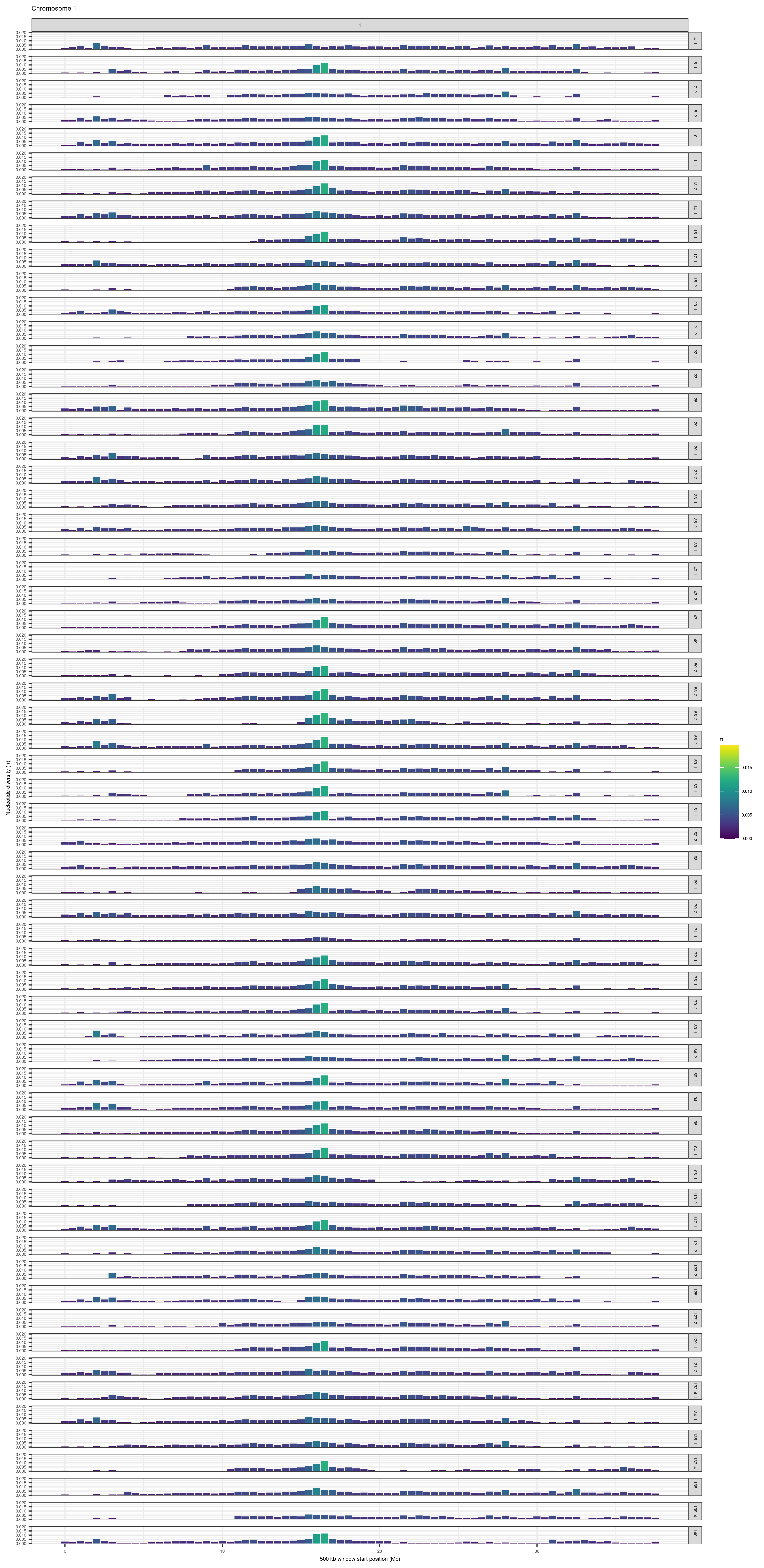

knitr::include_graphics(here::here("docs/plots/nucleotide_diversity/20211006_pi_per_chr/2.png"))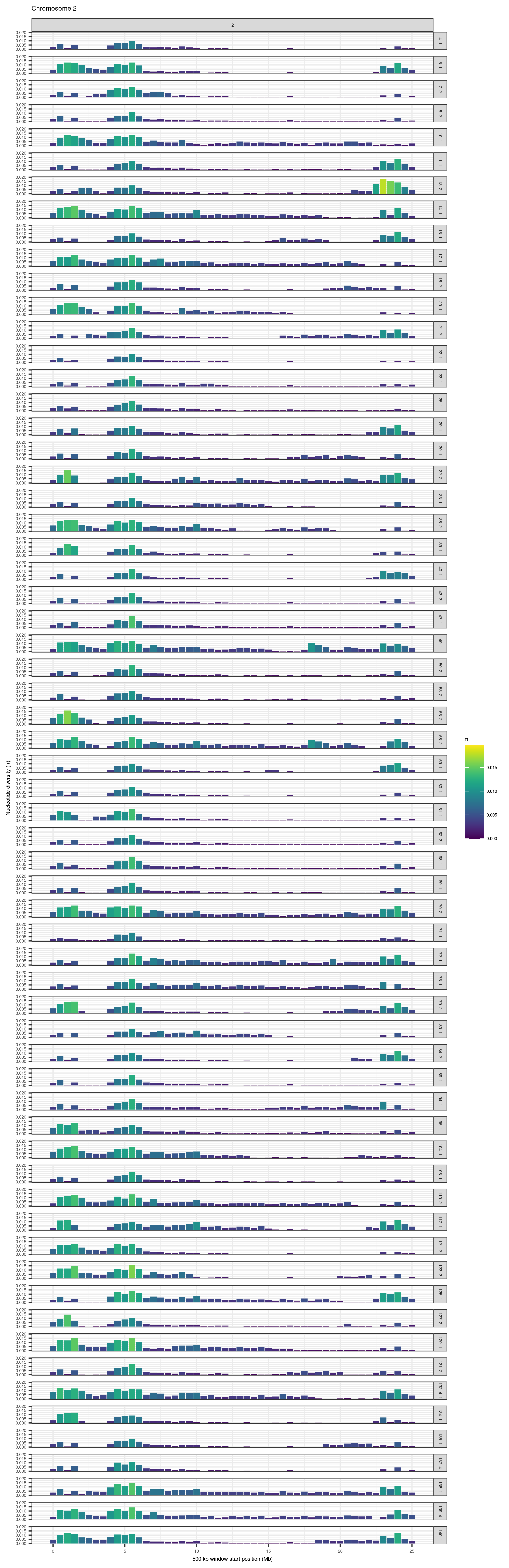

knitr::include_graphics(here::here("docs/plots/nucleotide_diversity/20211006_pi_per_chr/22.png"))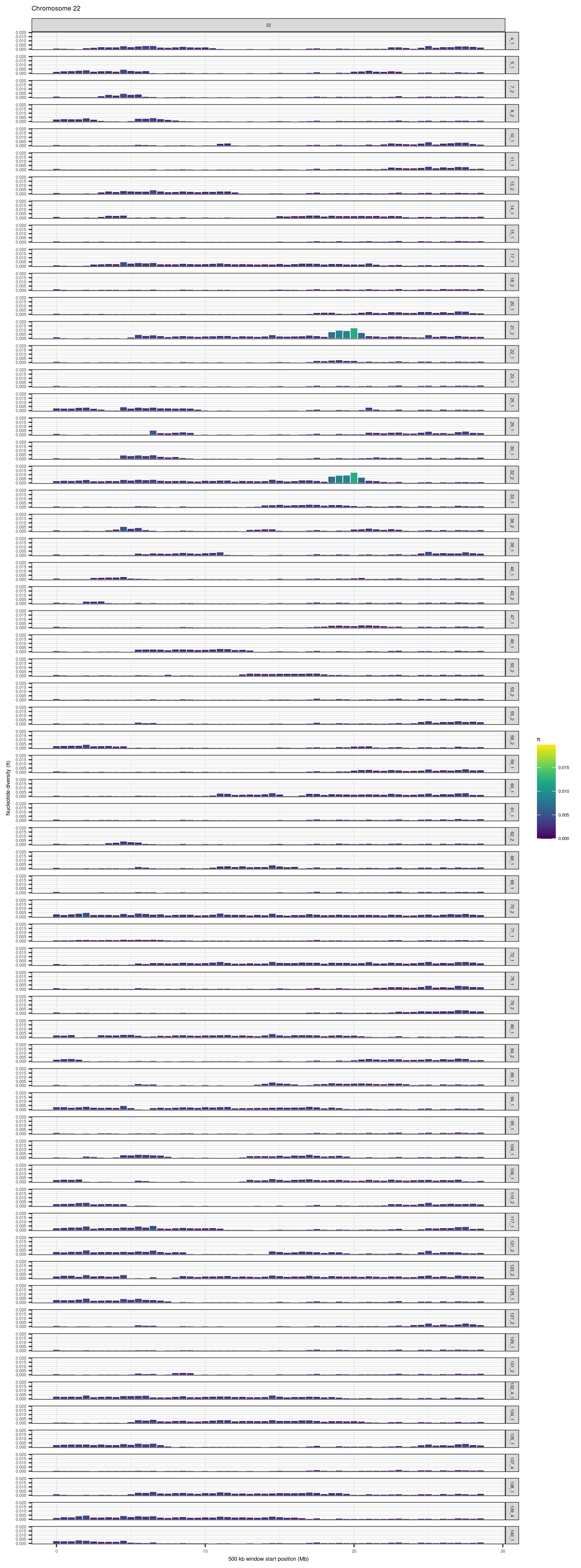

6.1.6 chr1 and 22 for supplementary figures

target_chrs = c(1, 22)
# Create plot
final_plot_df = mikk_df %>% 
  # Filter for target CHROM
  dplyr::filter(CHROM %in% target_chrs) %>% 
  # Create Mb column
  dplyr::mutate(Mb = (BIN_START - 1) / 1e6)
out_plot = final_plot_df %>% 
  ggplot() +
    geom_col(aes(Mb, PI, fill = PI)) +
    facet_grid(rows = vars(LINE), cols = vars(CHROM)) +
    theme_bw() +
    theme(text = element_text(size = 5)) +
    ylim(c(0, max(mikk_df$PI))) +
    xlab("500 kb window start position (Mb)") +
    ylab(expression(paste("Nucleotide diversity (", pi, ")", sep = ""))) +
    scale_fill_viridis(name = expression(pi), limits = c(0,max(mikk_df$PI)))

out_plot 

# Save
ggsave(here::here("docs/plots/nucleotide_diversity/20211013_chrs_1_22.png"),
       plot = out_plot,
       device = "png",
       width = 15,
       height = 20,
       units = "in",
       dpi = 400)

knitr::include_graphics(here::here("docs/plots/nucleotide_diversity/20211006_pi_per_chr/1.png"))

knitr::include_graphics(here::here("docs/plots/nucleotide_diversity/20211006_pi_per_chr/2.png"))

knitr::include_graphics(here::here("docs/plots/nucleotide_diversity/20211006_pi_per_chr/22.png"))

6.2 Investigate QC stats for sample MIKK10_1 to determine appropriate cutoffs

qc_file = "/hps/nobackup/birney/users/ian/mikk_genome/qc_stats/10_1.csv"

qc_df = readr::read_csv(qc_file,
                        col_names = c("CHROM", "POS", "DP", "MQ", "QD", "GQ"),
                        col_types = c("ciiddi")) %>% 
  # Filter for non-missing GQ
  dplyr::filter(complete.cases(GQ)) %>% 
  # Filter out MT
  dplyr::filter(CHROM != "MT") %>% 
  # Re-class CHROM
  dplyr::mutate(CHROM = factor(CHROM, levels = 1:24))

## Warning: One or more parsing issues, see `problems()` for details

6.2.1 Plot

qc_pairs = qc_df %>%
  # take sample to prevent over-plotting
  dplyr::slice_sample(n = 1e5) %>% 
  # create log10 for `DP`
  dplyr::mutate(LOG_10_DP = log10(DP)) %>% 
  GGally::ggpairs(.,
                  columns = c(7, 4, 5, 6),
                  lower = list(continuous = wrap("points", alpha = 0.2, size = 0.5),
                               combo = wrap("dot_no_facet", alpha = 0.4)))

qc_pairs

## plot: [1,1] [=====>----------------------------------------------------------------------------------------] 6% est: 0s
## plot: [1,2] [===========>----------------------------------------------------------------------------------] 12% est: 2s

## Warning in ggally_statistic(data = data, mapping = mapping, na.rm = na.rm, : Removing 1 row that contained a missing value

## plot: [1,3] [=================>----------------------------------------------------------------------------] 19% est: 2s

## Warning in ggally_statistic(data = data, mapping = mapping, na.rm = na.rm, : Removed 2 rows containing missing values

## plot: [1,4] [=======================>----------------------------------------------------------------------] 25% est: 3s
## plot: [2,1] [============================>-----------------------------------------------------------------] 31% est: 2s

## Warning: Removed 1 rows containing missing values (geom_point).

## plot: [2,2] [==================================>-----------------------------------------------------------] 38% est: 2s

## Warning: Removed 1 rows containing non-finite values (stat_density).

## plot: [2,3] [========================================>-----------------------------------------------------] 44% est: 2s

## Warning in ggally_statistic(data = data, mapping = mapping, na.rm = na.rm, : Removed 2 rows containing missing values

## plot: [2,4] [==============================================>-----------------------------------------------] 50% est: 2s

## Warning in ggally_statistic(data = data, mapping = mapping, na.rm = na.rm, : Removing 1 row that contained a missing value

## plot: [3,1] [====================================================>-----------------------------------------] 56% est: 1s

## Warning: Removed 2 rows containing missing values (geom_point).

## plot: [3,2] [==========================================================>-----------------------------------] 62% est: 1s

## Warning: Removed 2 rows containing missing values (geom_point).

## plot: [3,3] [================================================================>-----------------------------] 69% est: 1s

## Warning: Removed 2 rows containing non-finite values (stat_density).

## plot: [3,4] [=====================================================================>------------------------] 75% est: 1s

## Warning in ggally_statistic(data = data, mapping = mapping, na.rm = na.rm, : Removed 2 rows containing missing values

## plot: [4,1] [===========================================================================>------------------] 81% est: 1s
## plot: [4,2] [=================================================================================>------------] 88% est: 0s

## Warning: Removed 1 rows containing missing values (geom_point).

## plot: [4,3] [=======================================================================================>------] 94% est: 0s

## Warning: Removed 2 rows containing missing values (geom_point).

## plot: [4,4] [==============================================================================================]100% est: 0s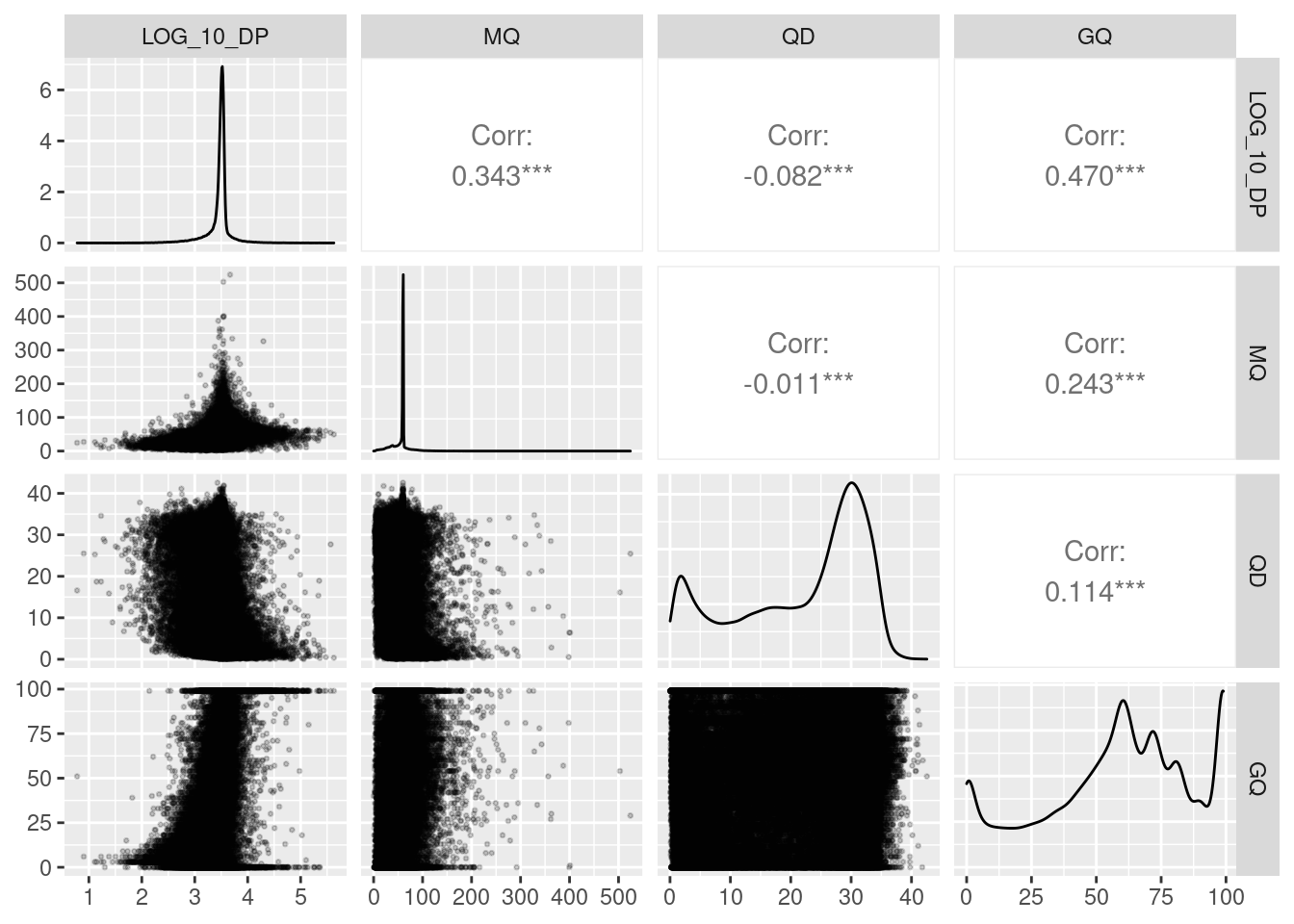

ggsave(here::here("docs/plots/nucleotide_diversity/20211006_qc_pairs.png"),
       plot = qc_pairs,
       device = "png",
       width = 10,
       height = 6,
       units = "in",
       dpi = 400)

How many calls have DP < x?

# Total variants
nrow(qc_df)

## [1] 27485882

# Number of variants with DP < x
length(which(qc_df$DP < 10))

## [1] 151

length(which(qc_df$DP < 20))

## [1] 723

length(which(qc_df$DP < 30))

## [1] 1823

length(which(qc_df$DP < 40))

## [1] 3378

So few!

Try GQ >= 40 & DP >= 40 & MQ >= 50.

6.3 Read in nucleotide diversity for filtered variants

6.3.1 MIKK

# Set location of data
in_dir = "/nfs/research/birney/users/ian/mikk_genome/nucleotide_divergence/mikk/filtered"

in_files_mikk_filt = list.files(in_dir, full.names = T)
mikk_list_filt = lapply(in_files_mikk_filt, function(IN_FILE) {
  # Read in 
  readr::read_delim(IN_FILE,
                    delim = "\t",
                    col_types = c("ciiid")) %>% 
    # Remove MT
    dplyr::filter(CHROM != "MT") %>% 
    # Make CHR an integer
    dplyr::mutate(CHROM = as.integer(CHROM)) %>% 
    # Create middle of bin
    dplyr::mutate(BIN_MID = ((BIN_END - BIN_START - 1) / 2) + BIN_START )
})
names(mikk_list_filt) = basename(in_files_mikk_filt) %>%
  str_remove(".windowed.pi")

# reorder
ordered_lines = tibble::tibble("LINE" = names(mikk_list_filt)) %>% 
  tidyr::separate(col = LINE, into = c("LINE", "SIB", "EXTRA"), sep = "_") %>% 
  dplyr::mutate(LINE = as.integer(LINE)) %>% 
  dplyr::arrange(LINE) %>% 
  tidyr::unite(col = "ORIGINAL", sep = "_", na.rm = T) %>% 
  dplyr::pull()

## Warning: Expected 3 pieces. Missing pieces filled with `NA` in 62 rows [1, 2, 3, 4, 5, 6, 7, 8, 9, 10, 11, 12, 13, 15, 16,
## 17, 18, 19, 20, 21, ...].

mikk_list_filt = mikk_list_filt[order(match(names(mikk_list_filt), ordered_lines))]

# Bind rows
mikk_df_filt = mikk_list_filt %>% 
  dplyr::bind_rows(.id = "LINE") %>% 
  # factor LINE to order
  dplyr::mutate(LINE = factor(LINE, levels = names(mikk_list_filt)))

6.3.2 Wild

# Set location of data
in_dir = "/nfs/research/birney/users/ian/mikk_genome/nucleotide_divergence/wild/filtered"

in_files_wild_filt = list.files(in_dir, full.names = T)
wild_list_filt = lapply(in_files_wild_filt, function(IN_FILE) {
  # Read in 
  readr::read_delim(IN_FILE,
                    delim = "\t",
                    col_types = c("ciiid")) %>% 
    # Remove MT
    dplyr::filter(CHROM != "MT") %>% 
    # Make CHR an integer
    dplyr::mutate(CHROM = as.integer(CHROM)) %>% 
    # Create middle of bin
    dplyr::mutate(BIN_MID = ((BIN_END - BIN_START - 1) / 2) + BIN_START )
})
names(wild_list_filt) = basename(in_files_wild_filt) %>%
  str_remove(".windowed.pi")

# Bind rows
wild_df_filt = wild_list_filt %>% 
  dplyr::bind_rows(.id = "LINE")

6.3.3 Combine

pi_df_filt = list("MIKK" = mikk_df_filt,
                  "WILD" = wild_df_filt) %>% 
  dplyr::bind_rows(.id = "POPULATION")

6.3.4 All chromosomes

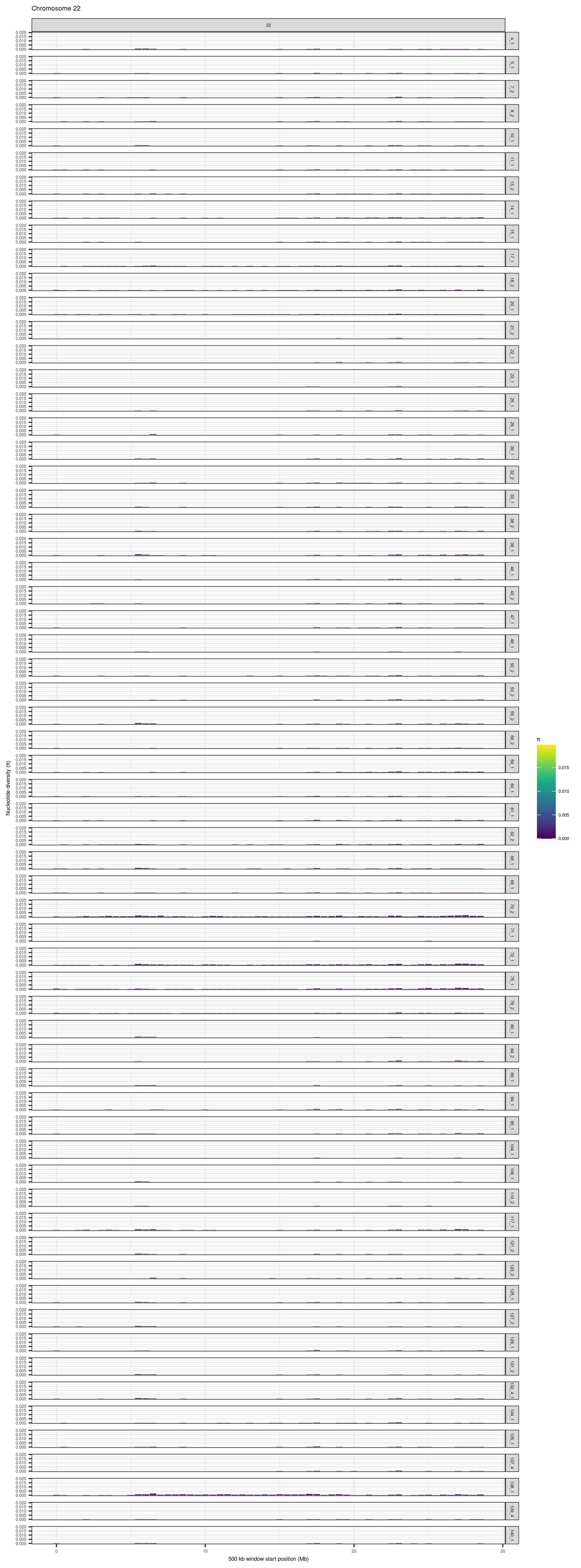
purrr::map(1:24, function(CHR){
    # Create plot
    plot_df = mikk_df_filt %>% 
      # Filter for target CHROM
      dplyr::filter(CHROM == CHR) %>% 
      # Create Mb column
      dplyr::mutate(Mb = (BIN_START - 1) / 1e6)
    
    out_plot = plot_df %>% 
      ggplot() +
        geom_col(aes(Mb, PI, fill = PI)) +
        facet_grid(rows = vars(LINE), cols = vars(CHROM)) +
        theme_bw() +
        theme(text = element_text(size = 5)) +
        ylim(c(0, max(mikk_df$PI))) +
        xlab("500 kb window start position (Mb)") +
        ylab(expression(paste("Nucleotide diversity (", pi, ")", sep = ""))) +
        ggtitle(paste("Chromosome ", CHR, sep = "")) +
        scale_fill_viridis(name = expression(pi), limits = c(0,max(mikk_df$PI)))
        
    
    # Adjust width dimensions of plot based on length of chromosome
    w_dim = mikk_df_filt %>% 
      dplyr::filter(CHROM == CHR) %>% 
      dplyr::mutate(Mb = (BIN_START - 1) / 1e6) %>% 
      dplyr::pull(Mb) %>% 
      max(.)
    w_dim = w_dim * 0.26
    # Save
    ggsave(here::here("docs/plots/nucleotide_diversity/20211006_pi_per_chr_filtered", paste(CHR, ".png", sep = "")),
           plot = out_plot,
           device = "png",
           width = w_dim,
           height = 20,
           units = "in",
           dpi = 400)
})

knitr::include_graphics(here::here("docs/plots/nucleotide_diversity/20211006_pi_per_chr_filtered/1.png"))
knitr::include_graphics(here::here("docs/plots/nucleotide_diversity/20211006_pi_per_chr_filtered/22.png"))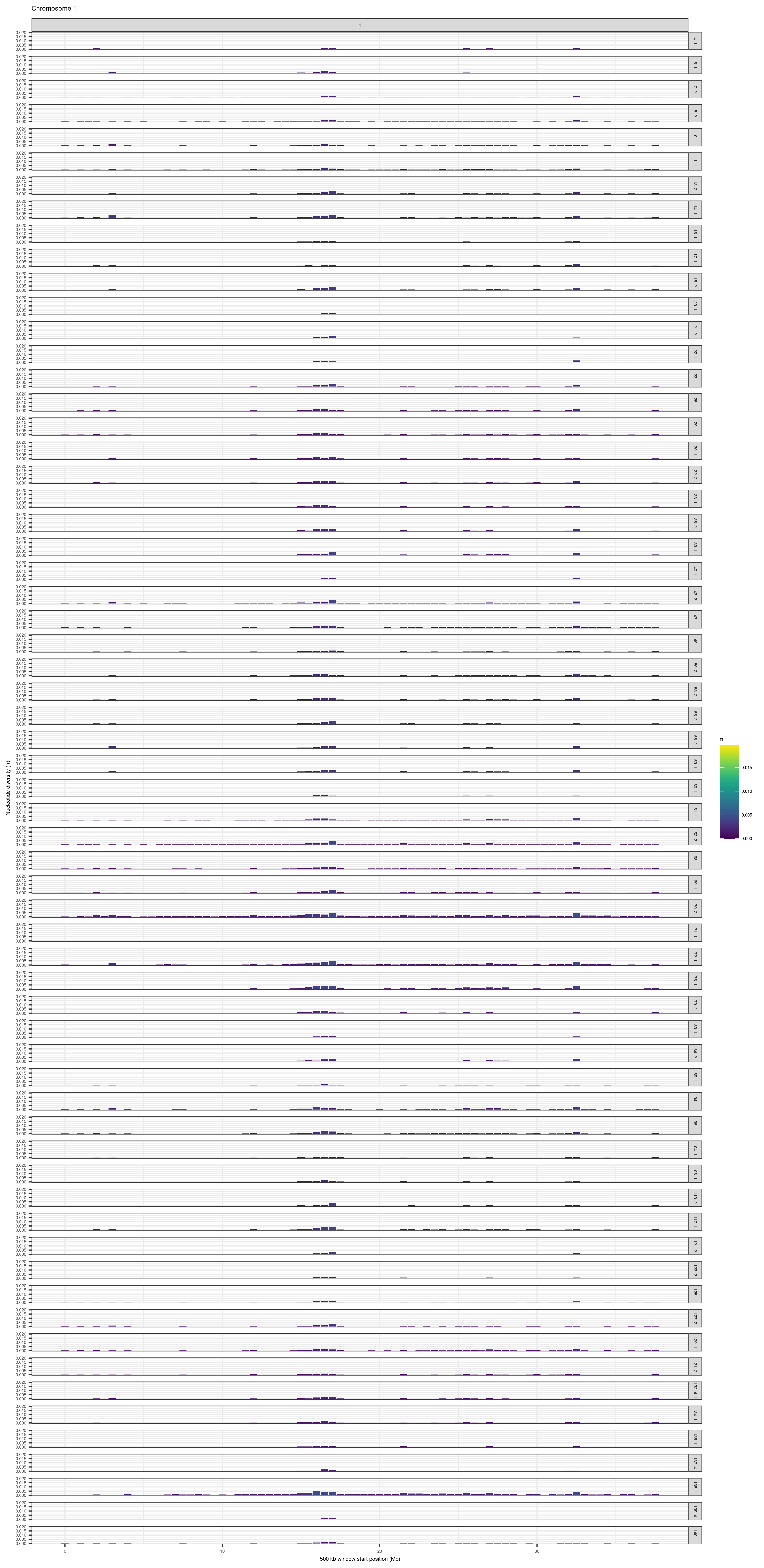

6.3.5 Boxplots

# source `darker` function
source("https://gist.githubusercontent.com/brettellebi/c5015ee666cdf8d9f7e25fa3c8063c99/raw/91e601f82da6c614b4983d8afc4ef399fa58ed4b/karyoploteR_lighter_darker.R")

# What is the median for MIKK v WILD?
pi_df_filt %>% 
  dplyr::group_by(POPULATION) %>% 
  dplyr::summarise(MEAN_PI = mean(PI, na.rm = T),
                   MEDIAN_PI = median(PI, na.rm = T))

## # A tibble: 2 × 3
##   POPULATION  MEAN_PI MEDIAN_PI
##   <chr>         <dbl>     <dbl>
## 1 MIKK       0.000298  0.000082
## 2 WILD       0.000253  0.00008

# Together
mikk_wild_boxplot = pi_df_filt %>% 
  ggplot() +
    geom_violin(aes(POPULATION, log10(PI), colour = POPULATION, fill = POPULATION)) +
    geom_boxplot(aes(POPULATION, log10(PI), colour = POPULATION, fill = POPULATION), width = 0.1) +
    theme_bw() +
    scale_fill_manual(name = "Population", values = pal) +
    scale_colour_manual(name = "Population", values = darker(pal, 80)) +
    ylab(expression(paste(log[10], "(", pi, ")", sep = ""))) +
    ggtitle("Nucleotide diversity in 500 kb bins (MAPQ >= 50 & GQ >= 40 & DP >= 40 )")

mikk_wild_boxplot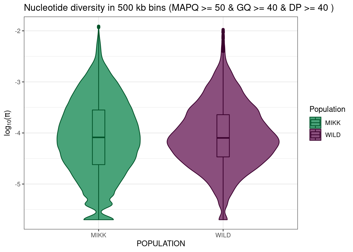

ggsave(here::here("docs/plots/nucleotide_diversity/20211006_mikk_wild_boxplot.png"),
       plot = mikk_wild_boxplot,
       device = "png",
       width = 8,
       height = 6,
       units = "in",
       dpi = 400)

6.3.5.1 Take only 7 MIKK samples

set.seed(13)
# Pull out 7 random MIKK samples
mikk_random_samples = pi_df_filt %>% 
  dplyr::filter(POPULATION == "MIKK") %>% 
  dplyr::distinct(LINE) %>%
  dplyr::slice_sample(n = 7) %>% 
  dplyr::pull(LINE)
  
# Plot
mikk_wild_boxplot_samp = pi_df_filt %>% 
  dplyr::filter(POPULATION == "WILD" | LINE %in% mikk_random_samples) %>% 
  ggplot() +
    geom_violin(aes(POPULATION, log10(PI), colour = POPULATION, fill = POPULATION)) +
    geom_boxplot(aes(POPULATION, log10(PI), colour = POPULATION, fill = POPULATION), width = 0.1) +
    theme_bw() +
    scale_fill_manual(name = "Population", values = pal) +
    scale_colour_manual(name = "Population", values = darker(pal, 80)) +
    ylab(expression(paste(log[10], "(", pi, ")", sep = ""))) +
    ggtitle("Nucleotide diversity in 500 kb bins (MAPQ >= 50 & GQ >= 40 & DP >= 40 )\n7 MIKK lines & 7 wild Kiyosu samples")

mikk_wild_boxplot_samp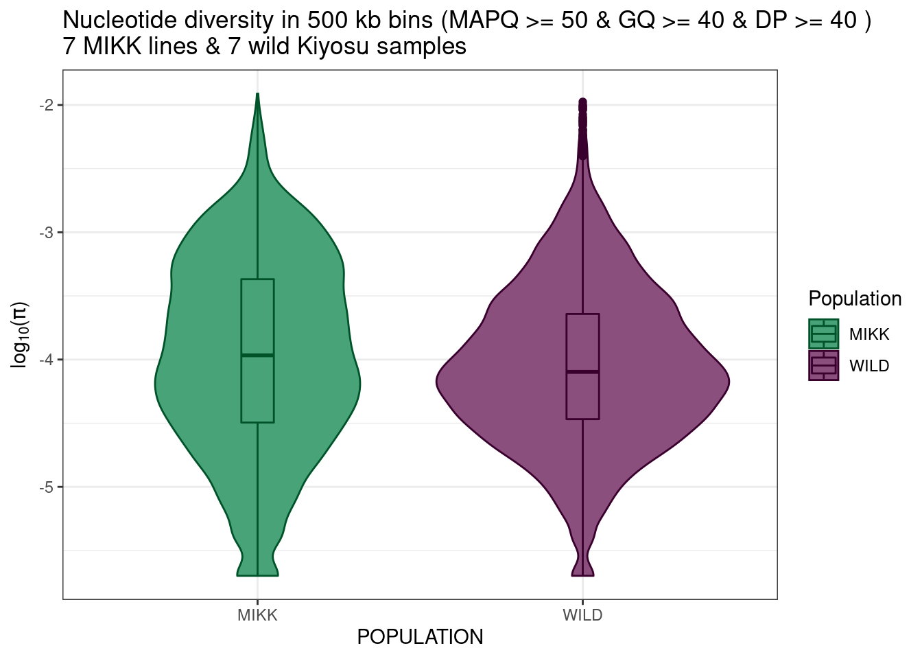

ggsave(here::here("docs/plots/nucleotide_diversity/20211011_mikk_wild_boxplot_sampled.png"),
       plot = mikk_wild_boxplot_samp,
       device = "png",
       width = 8,
       height = 6,
       units = "in",
       dpi = 400)

6.3.5.2 Faceted

mikk_wild_boxplot_facet = pi_df_filt %>% 
  ggplot() +
    geom_violin(aes(POPULATION, log10(PI), colour = POPULATION, fill = POPULATION)) +
    geom_boxplot(aes(POPULATION, log10(PI), colour = POPULATION, fill = POPULATION), width = 0.05) +
    theme_bw() +
    scale_fill_manual(name = "Population", values = pal) +
    scale_colour_manual(name = "Population", values = darker(pal, 80)) +
    ylab(expression(paste(log[10], "(", pi, ")", sep = ""))) +
    facet_wrap(vars(CHROM), nrow = 4, ncol = 6) +
    guides(colour = "none", fill = "none") +
    ggtitle("Nucleotide diversity in 500 kb bins (MAPQ >= 50 & GQ >= 40 & DP >= 40 )")

mikk_wild_boxplot_facet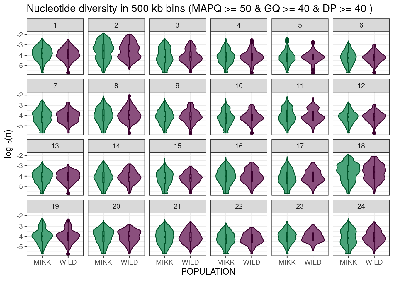

ggsave(here::here("docs/plots/nucleotide_diversity/20211006_mikk_wild_boxplot_facet.png"),
       plot = mikk_wild_boxplot_facet,
       device = "png",
       width = 8,
       height = 6,
       units = "in",
       dpi = 400)

Nucleotide diversity

2022-02-09

1 Load libraries

2 Snakemake pipeline to process VCF and extract data

3 Process data

3.1 Read in data

3.1.1 MIKK

3.1.2 Wild Kiyosu

4 Karyoplot

4.1 Set up scaffold

4.2 Plot

4.2.1 Compare effect of bin width on noise

5 Circos

5.1 Get repeats data

5.2 Calculate proportion of bin covered by repeats

5.2.1 Bin intevals

5.2.2 Repeats

5.2.3 Find quantity of repeats overlapping bins

5.3 Read in mapping quality scores

5.4 Bind data frames

5.5 Pairs plot

5.6 Circos

5.6.1 1 Mb

5.6.1.1 Rearrange data frames

5.6.1.2 Plot

5.6.2 500 Kb

5.6.2.1 Create data frame

5.6.2.1.1 Repeats

5.6.2.1.2 MQ

5.6.2.1.3 Final

5.6.3 Mean and median Pi

5.6.3.1 63 MIKK samples v 7 wild Kiyosu

5.6.3.2 7 MIKK samples v 7 wild Kiyosu

6 Per-individual

6.1 Read in data

6.1.1 MIKK

6.1.2 Wild

6.1.3 Combine

6.1.4 Boxplot

6.1.5 All chromosomes

6.1.6 chr1 and 22 for supplementary figures

6.2 Investigate QC stats for sample MIKK10_1 to determine appropriate cutoffs

6.2.1 Plot

6.3 Read in nucleotide diversity for filtered variants

6.3.1 MIKK

6.3.2 Wild

6.3.3 Combine

6.3.4 All chromosomes

6.3.5 Boxplots

6.3.5.1 Take only 7 MIKK samples

6.3.5.2 Faceted